Single Linkage Clustering Heuristic
Explaining the magic fudge in Mapper.
Background
A few months back I attended a couple of seminars by Gunner Carlsson talking about topological data analysis, and discussed some methods they employ at Ayasdi. Given my background in mathematics I thought it was quite nice to see some concrete applications of some rather abstract theory. In addition to this, their topology based analysis methods seem to be succesful with bioinformatical data where other methods fail.
This first paper about the method describes it quite well, and on the groups website they are also hosting a Matlab script which they used for the applications in that first paper. This scientific report gives a very nice summary of capabilities of topology based data analysis.
Using their refined implementation of the method on your data means contacting them and sending them your data to run their analysis on.
Therefore I thought a nice evening project would be to reimplement the Matlab script in Python, so it can be easily run anywhere, and eventually optimize the implementation somewhat.
A great start would be at the [upcoming Seqahead Hackathon] (http://seqahead.cs.tu-dortmund.de/meetings:2013-06-hackathon), where I’d hoped to perhaps get some collaboration.
Mapper basics
Just extremely briefly (see the scientific report or paper for details), the
basic idea of Mapper is to divide the space of the data in to sections.
Within these sections clustering is performed, these clusters are then combined
depending on overlaps to form a graph which reveals a “shape” of the data.
Single Linkage Clustering
In the Matlab implementation of Mapper the authors use single linkage
clustering. Briefly, single linkage clustering means initially taking every
object as a cluster on its own, then pairwise link together “clusters” which
are the closest to each other. This is repeated until the algorithm is left
with one single cluster.
Software performing this kind of clustering usually returns a representation of the tree being built throughout the clustering, with the intermediate distances between clusters in each step preserved.
Mysteries in the Matlab implementation
When reading the Matlab implementation one comes across the parameter
magicFudge. This is described in the comments of the script.
%  magicFudge: The number of histograms to divide each homology plot into
%              Increase this number if you expect to see more clusters
%              and decrease it if you are seeing more clusters.
%              Default : 10
Heuristic for number of clusters
This is further explained in the paper (page 5).
Now, to find the number of clusters we use the edge length at which each cluster was merged. The heuristic is that the interpoint distance within each cluster would be smaller than the distance between clusters, so shorter edges are required to connect points within each cluster, but relatively longer edges are required to merge the clusters. If we look at the histogram of edge lengths in C, it is observed experimentally, that shorter edges which connect points within each cluster have a relatively smooth distribution and the edges which are required to merge the clusters are disjoint from this in the histogram. If we determine the histogram of C using k intervals, then we expect to find a set of empty in- terval(s) after which the edges which are required to merge the clusters appear.
The authors also points out problems with this approach.
Although this heuristic has worked well for many datasets that we have tried, it suffers from the following limitations: (1) If the clusters have very different densities, it will tend to pick out clusters of high density only. (2) It is possible to construct examples where the clusters are distributed in such a way such that we re- cover the incorrect clustering. Due to such limitations, this part of the procedure is open to exploration and change in the future.
While I was reading the paper, I didn’t think much about this heuristic, but when trying to implement the method, it got me fairly confused.
I figured it would be nice to try the heuristic out and see how well it performs.
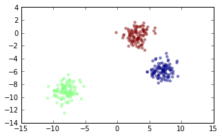
First we want to simulate some data, there’s a nice function in scikits-learn
to generate blobs of data (clusters): sklearn.datasets.make_blobs. First
generate some clusters.
from sklearn import datasets
num_clusters = 3
X, y = datasets.make_blobs(n_samples=N, centers=num_clusters)
(Throughout this post, I will omit commands for creating plots, but it can all be viewd in this IPython notebook.)
To perform single linkage clustering, we need a distance matrix between all points in the data set.
from scipy.spatial import distance
d = distance.cdist(X, X)
Then we can use, e.g. this new fastcluster package to perform the clustering.
import fastcluster
Z = fastcluster.linkage(d, method='single')
This creates the linkage Z, a (num_points - 1, 4)-shaped array where the
distance between Z[i, 0] and Z[i, 1] is Z[i, 2].
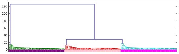
This graph contains a dendrogram representation of the linkage.
In Mapper they also add the longest distance from the distance matrix to the
array of inter cluster distances.
lens = np.zeros(Z.shape[0] + 1)
lens[:-1] = Z[:, 2]
lens[-1] = d.max()
They also introduce the notion of calling this collection of distances a “lens”. I like this as it invokes the idea of “unfocusing” the view of the data to see the overall shape.
Now just look at the histogram of distances.
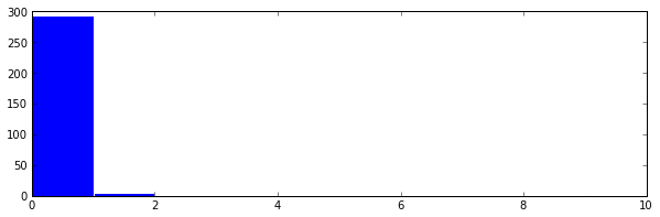
This finds one cluster, as can be seen by doing the following.
z = np.nonzero(hst == 0)[0]
hst[z[0]:len(hst)].sum()

Out[613]: 1
It’s pretty impossible to see, but this cluster has the distances in the 9th
bin in the histogram. This is obviously wrong, since we knew beforehand that we
made three clusters in this example. Thus we should “focus” the lens by
increasing the magicFudge, in this case I increase it to 64.
magic_fudge = 64
hst, _ = np.histogram(lens, bins=magic_fudge)

z = np.nonzero(hst == 0)[0]
hst[z[0]:len(hst)].sum()

Out[632] 3
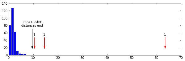
Here we see the pattern discussed in the paper quite clearly. A nice almost normal distribution of small distances, breaking at the 9th bin (black arrow), followed by three bins at various locations with a single distance in.
Now to the issue that motivated this blog post: It took my many tries of
generating example clusters, as well as trying different magicFudge-values
for this last histogram.
Testing the heuristic
To see how the heuristic performed, I wrote some code that randomly generates
between one and six clusters, performs the cluster count using nine different
magicFudge-values, and collects how many times for each value the heuristic
found the correct number of clusters.
magic_fudge_settings = [8, 16, 25, 32, 50, 64, 100, 128, 256]
hit_counts = [0] * len(magic_fudge_settings)
n_tests = 500
for i in range(n_tests):
    true_num_clusters = random.randint(1, 6)

    X, _ = datasets.make_blobs(n_samples=300, centers=true_num_clusters)

    d = distance.cdist(X, X)
    Z = fastcluster.linkage(d, method='single')
    lens = np.zeros(Z.shape[0] + 1)
    lens[:-1] = Z[:, 2]
    lens[-1] = d.max()

    for j, magic_fudge in enumerate(magic_fudge_settings):
        hst, _ = np.histogram(lens, bins=magic_fudge)
        z = np.nonzero(hst == 0)[0]
        if len(z) == 0:
            num_clusters = 1
        else:
            num_clusters = hst[z[0]:len(hst)].sum()

        if num_clusters == true_num_clusters:
            hit_counts[j] += 1
Results
Are best summarized with the following plot.

These results are quite bad in my opinion. However, when using this process to find clusters in order to make a graph of connections between them, it is probably not that important to be accurate. Just as long as enough overlapping clusters are found we will end up with a nice network that describes the data. But I very much doubt this is the cluster counter method used in the production implementation at Ayasdi.