Unscaling scaled counts in scRNA-seq data

It is always good to compare your measurements with measurements others have done before you. This way you get a feeling for expected outcomes, expected variation in measurement, etc.

In single cell RNA-seq, I tend to apply this principle by looking at a lot of published data, to see how the properties of data in general correspond to data that I’m analyzing for the sake of scientific investigation.

Single cell RNA-seq data consists of observed counts of molecules generated from different genes in different cells. Sometimes however, authors only publish counts that have been scaled. One very popular unit is CPM, counts per million, where the counts in each cell is divided by the sum of counts, then multiplied by a million. Recently I have also noticed data with similar scaling to 10,000 or 100,000, or to a median across the data set.

To compare data from different sources, it is easier to interpret differences if you know the per-cell total counts. It allows you to think of the counts in the data in the context of exposure. I recently wanted to look at some 10X data, but it turned out the expression matrix did not consist of counts.

Looking at the mean-variance relation for all the genes in the data it was clear that they had been log-transformed.

Even after exponentiating the expression levels, they were not integers. However, looking at the sum of expression levels in each cell it could easily be seen that the counts had been scaled to 10,000 counts per cell.

One would think that this is a lossy transformation: we wouldn’t know how large the magnitudes in a cell were before division. However, the very problem with scaling of counts means we can recover the value used to scale the cell.

It’s not clear if this is a biological property or a property of the measurement process, but out of the 20,000 or so genes, in scRNA-seq data of any given cell, the vast majority of genes will have 0 counts. Follows by a substantial number of genes with 1 counts, followed by a slightly smaller number of genes with 2 counts, etc.

Since the scaling by division just changes the magnitude of the counts, but not the discrete nature, the most common value will correspond to 0, the second most common value to 1, etc. This plot of a few random cells make this relation clear.

Just looking at the second most common value in the histogram of a cell will give us the factor used to scale the cell! (For the sake of some robustness, I used several ranks in the histogram and the corresponding scaled counts and fitted the scaling factor with least squares, but the difference from the second most common value was all in all negligible).

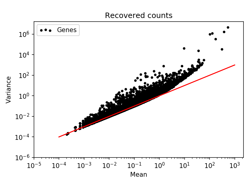
By simply multiplying the cells by the identified scaling factors, the true counts are recovered. After un-scaling, the typical relation between total count and detected genes is clear, and the negative binomial mean-variance relation for genes is apparent.

I wanted to write about this, because the fact that it is possible to recover the original counts after scaling indicates that just scaling the counts is not sufficient for normalization. The properties if discrete counts are still present in the data, and will be a factor in every analysis where these scaled counts are used. It will make interpretation hard, since the relation between magnitude and the probability of generating values magnitude will not be tied to each other as clearly as with counts.

Notebook with this analysis is available here.