
Causal temperatures

Time is special. It only moves in one direction. Seeing one thing happen before another thing carries a lot of information. The second thing cannot have caused the first thing to happen.
For a long time, I have believed that the lack of high resolution temporal data of gene expression has been a bottleneck in learning accurate regulatory networks of transcriptional regulation (this was the basis for my research program before going to the therapeutics industry). Since technologies for these measurement don’t exist, I have kept an eye out for other, comparable, datasets to learn how analysis methods for temporal causal inference works.
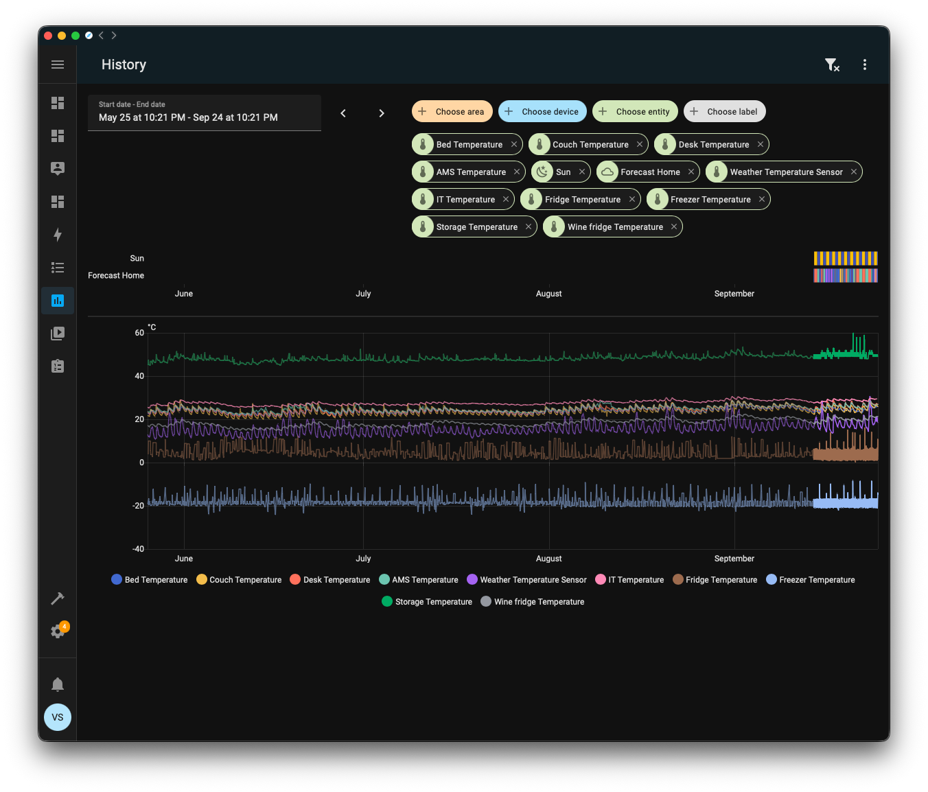
A while ago a got a Home Assistant server and connected multiple thermometers throughout my non-air conditioned apartment to it. Sensors, like thermometers, are recorded over time in Home Assistant, allowing you to look up history at high resolution for long periods of time.
This seemed like an interesting opportunity to test out Granger analysis, a classical method to identify causality from time series data.
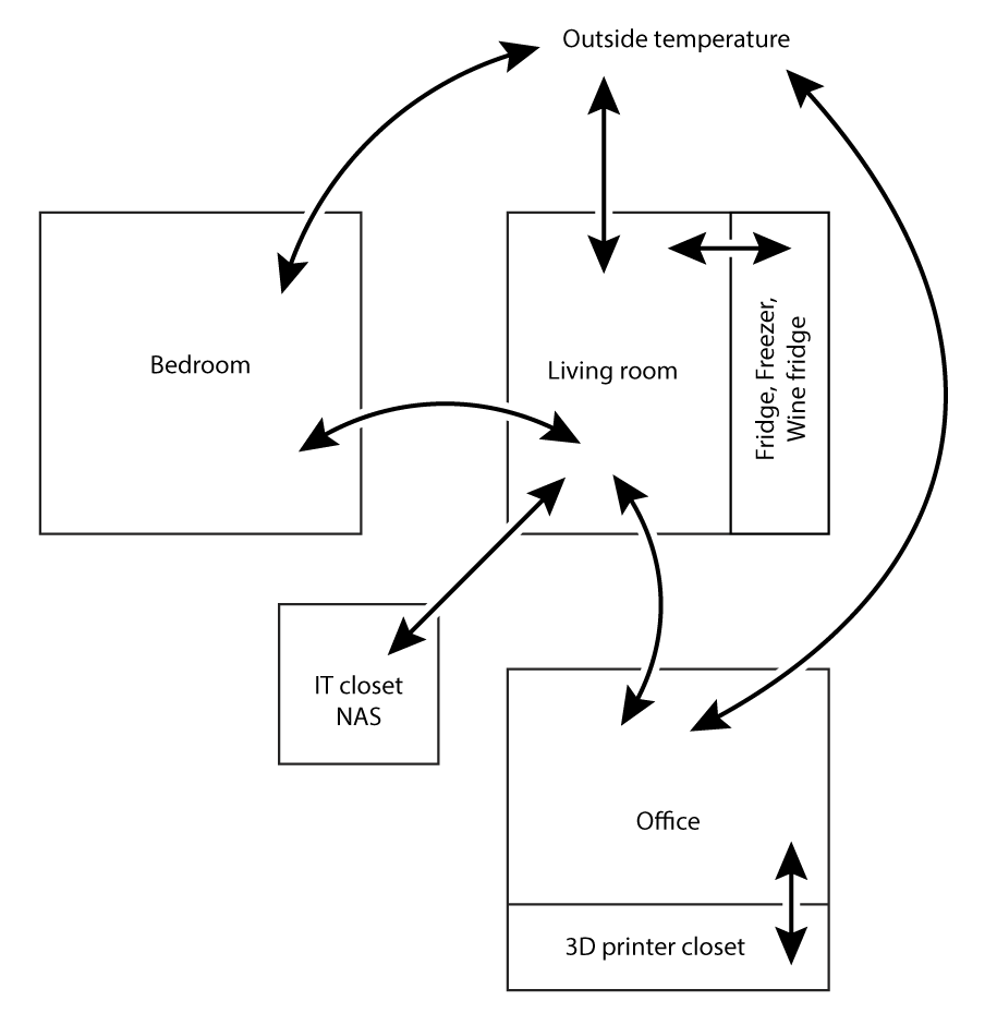
Not having an HVAC system, I have a pretty good idea of how air flows between the rooms. This should determine heat exchange between them. Which rooms heat up first throughout the day and transport heat to the other rooms is not obvious though.
I downloaded the temperature sensor data from Home Assistant for the last few months, comprising 37,110 measurements from ten thermometers.
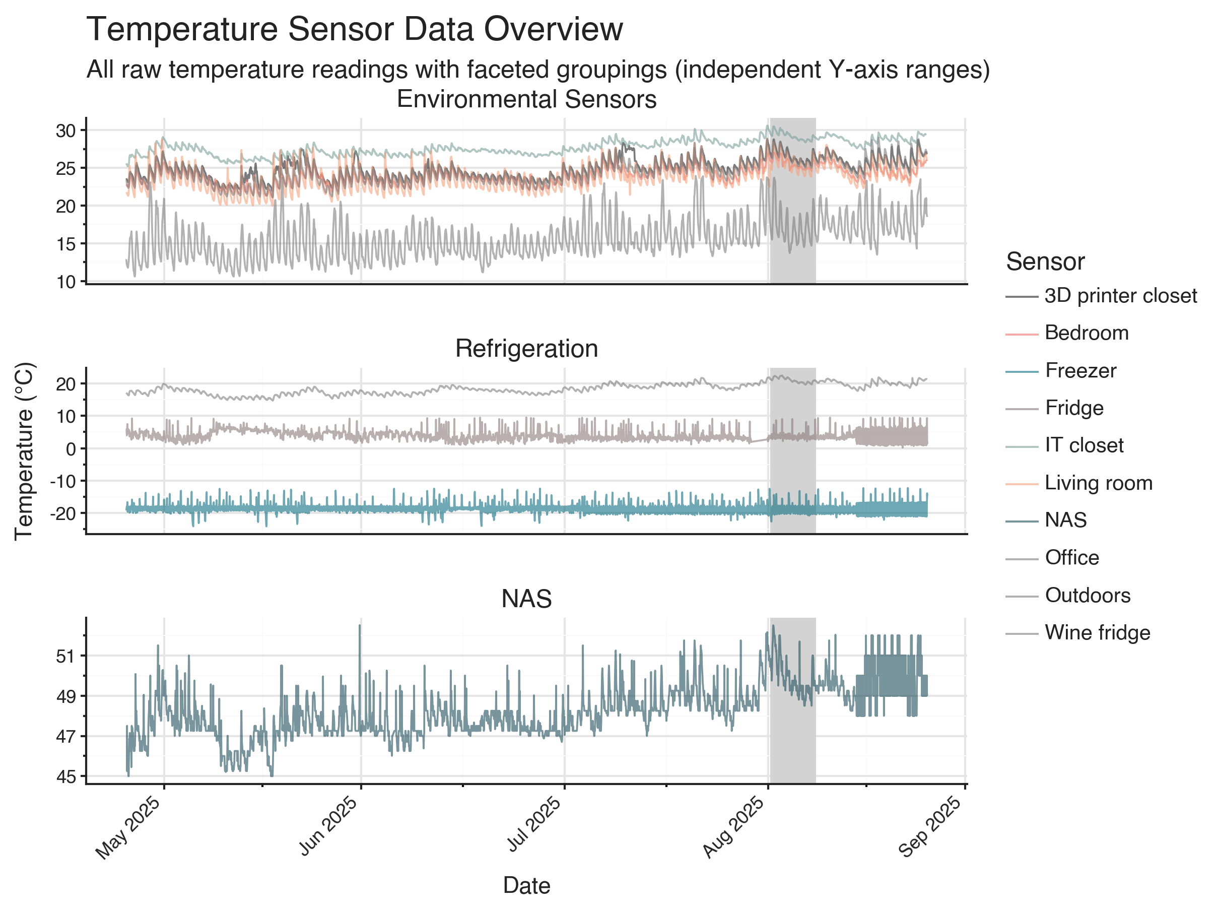
Longer term seasonal trends can be seen through correlated increases in average temperature across ambient air thermometers. When looking at the full dataset, it is hard to daily fluctuations in temperature.
I have split up the thermometers into three categories: environmental sensors, refrigeration, and NAS. Environmental sensors measures the temperature of the air in the rooms or closets. Refrigeration thermometers measures the temperatures in fridges, and should (ideally) not be affected by room temperatures, and can be thought of a negative controls for a causal analysis. NAS is the temperature of my NAS which is hidden away in an IT closet. The temperature of the NAS is determined by the load as it is being used.
The oscillatory temperature changes in the fridges is due to the defrost cycle. Modern fridges and freezers vary the temperature to prevent frost buildup. This is why labs need to buy special, pricier, -20 freezers which maintains temperature more consistently.
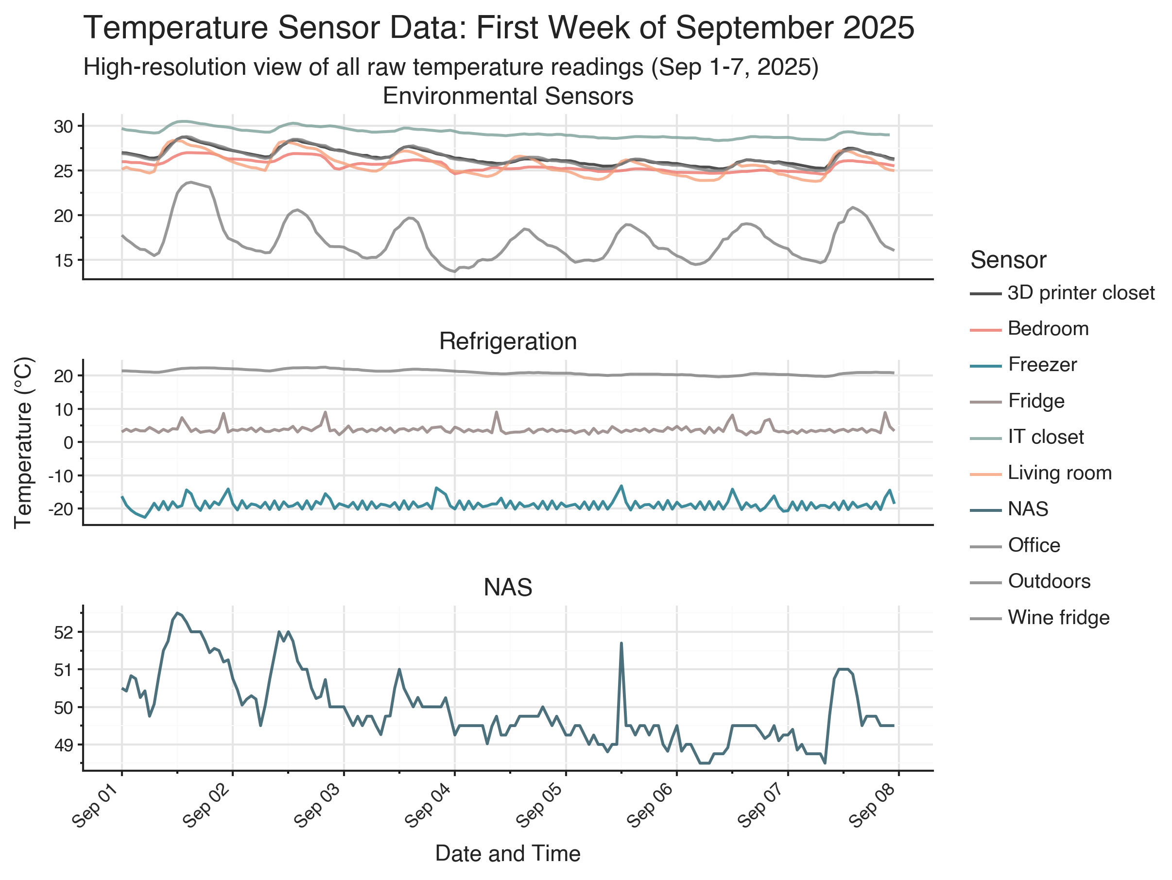
If you look closely at the environmental sensors, you might see that temperatures in some rooms peak before the temperature in other rooms. This property is what we’re hoping to use to learn directionality in heat transfer between rooms.
The classical method for this is Granger analysis. The idea is that you fit two models to your data: one simple autoregressive model,
and one bivariate autoregressive model,
where x are measurements from the potentially causal source. The null hypothesis, that x does not cause y, means that all beta coefficients are 0. Or, in other words, predictions when including x-values do not improve upon using only y-values.
The models can be compared using an F-statistic that compares the residual sum of squares for the two different models:
The simple autoregressive model is restricted since it uses a subset of the predictors available for the bivariate autoregressive model which also includes potentially causal measurements.
In the example above, the top panel uses three previous time points of office temperatures to predict temperature at a given time point, while the bottom panel can also use temperatures from three prior time points from the living room. The qualitative difference in predictions are hard to see by eye in the figure, but it has an F-statistic of 210, corresponding to an error reduction from an RMSE of 0.0970°C to an RMSE of 0.0671°C.
To build a causal network, we can pairwise fit these models to all possible combinations of temperature sensors, meaning 10 * 9 = 90 possible pairs.
There are some additional implementation details for the analysis.
To avoid spurious correlations from seasonality, models are fitted to first differences of the temperatures:
We also perform the analysis with multiple lag orders, between one and five hours at one-hour increments. That is, we fit one model using only one hour prior as predictor, another model with one and two hours prior as predictor, etc., up to five hours. The hourly intervals and limiting to five hours was chosen based on it being plausible for temperatures to change at these time scales.
After fitting all the models and getting all the F-statistics, we can use them to visualize the causal graph of how temperature flows through the apartment based on the sensor data.
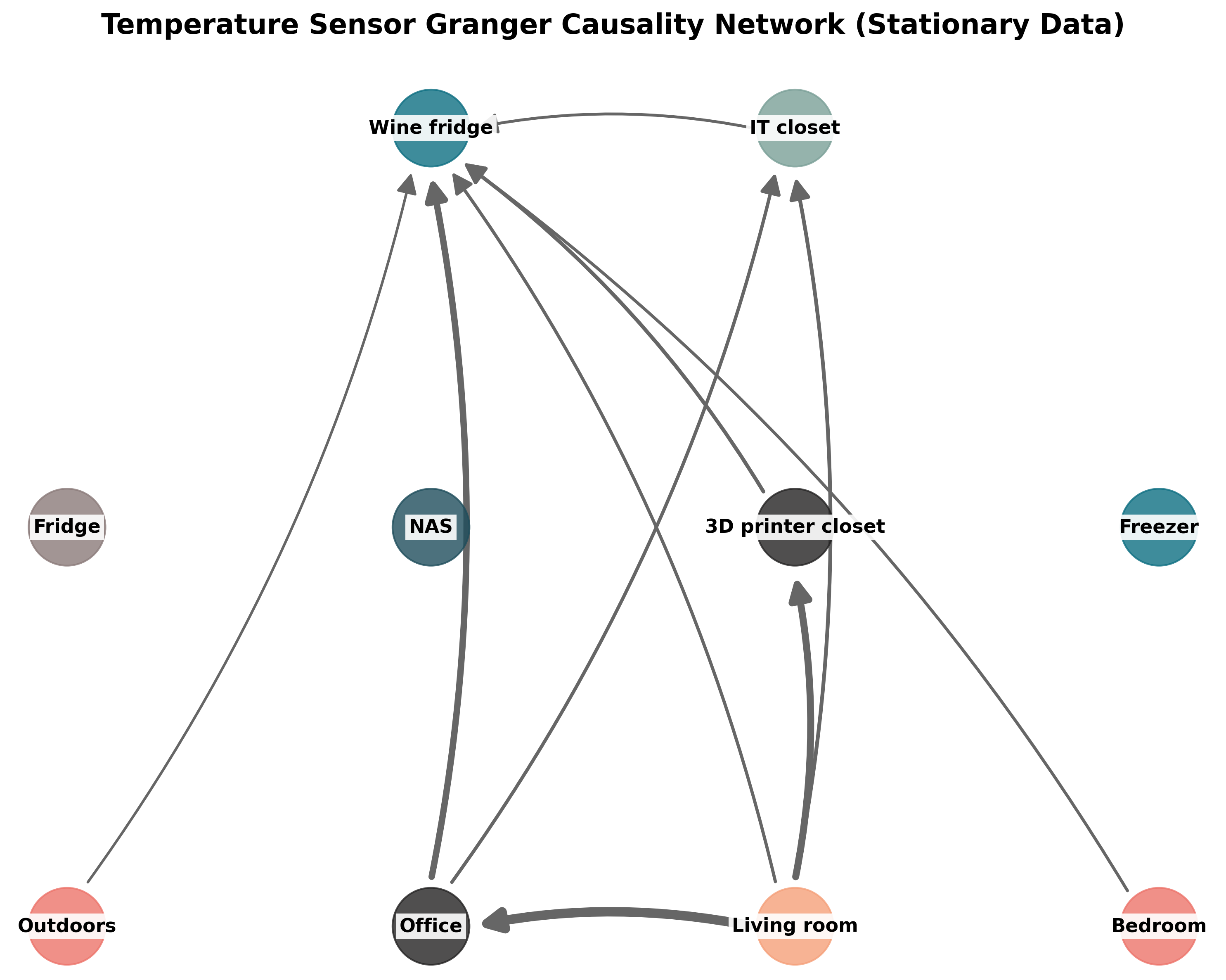
This diagram only shows relations with F-statistics larger than 400, a very strict threshold corresponding to a p-value of about 10^-85. Almost all relations between sensors pass a p-value threshold of 0.05. Since we have a very large number of observations, the test is powered to detect extremely small potential causes in a null hypothesis framework, and it is probably more productive to think about strength of evidence rather than null hypothesis significance testing.
The strongest link is from the living room to the office, which is believable. On the other hand, the 3D printer closet is physically located inside the office, and we are finding a stronger causal link between the living room and the 3D printer closet than from the office to the 3D printer closet. This seems like a false positive.
I would have expected the outdoors temperature to be a strong predictor throughout the system, but it’s not unreasonable that it’s not directly causal: sunlight hitting the apartment is likely to heat up the rooms before the outside temperature rises.
The lack of sunlight as a predictor is a general issue with the analysis. When there is an unobserved underlying causal factor, Granger analysis tend to produce false positive results. It is pretty likely that sunlight directly affects three of the rooms acting as a hidden confounder.
The wine fridge is affected by a lot sources. This is somewhat believable, because wine fridges are usually of much lower quality than standard fridges and don’t maintain consistent temperature well. It is not very believable that the IT closet or the 3D printer closet temperatures directly affect the temperature of the wine fridge; they should at least act through the office or living temperatures.
This highlights another shortcoming of this strategy. We are simply extracting the pairwise causal results. If there is an intermediate node, we are not testing if mediation through that node better explains the system than direct connections. Mediation should be visible in the system though, by triplets of nodes A, B, C being connected as A → B, A→ C, B → C, if A causes C mediated through B.
In addition to missing sunlight, other potential interventional factors like opening windows or cooking or running the 3D printer are not captured here. Though, I don’t do those very often, so I don’t think they affect the data at the majority of the time points.
Takeaways
Compared to the kind of data that can be generated for gene expression, this data is extremely high resolution, has an enormous amount of observations, and very little observational noise. The system is also very small compared to transcriptional regulation. But even with this data, accurately identifying a causal network is challenging.
It leaves me a bit pessimistic about the potential to identify transcriptional regulatory networks even with measurement technologies that currently don’t exist.
Granger analysis is a classical method that has been around for over half a century. Shortcomings of Granger analysis are well-known. I was hoping to find modern alternatives, and in the last few years the statistics community has had a large focus causality identification. There are many new methods and strategies, but to my surprise they tend to not make use of temporal information.
Scripts and data for this post are available on Github.
From around the web
