
Riemannian Newton iteration for Rayleigh quotients on the sphere


In the above figure, each point is in initial value which will be converge to different eigenvectors of an orthogonal 3x3 matrix. The above figure is the equivalent of a Newton fractal, but applied to Rayleigh quotient iteration on a sphere. This post will go through an explanation of the figure, and the numerical method on the sphere, which can be applied to any manifold.
Rayleigh quotients and Eigenvectors
Given a Hermetian matrix M and a vector x the Rayleigh quotiend is defined by
For the sake of this text, let us limit ourselves to looking at M=ATA which are covariance matrices of some data matrix A. This implies that M has unique real values eigenvalues. In addition we know that the eigenvectors of M will be orthogonal.
Using these eigenvectors as a basis, let us express an arbitrary vector x as a linear combination of eigenvectors.
Now we have that
since eigenvectors are orthogonal. Additionally, we see that the sum in the last equality will be minimized when x is orthogonal to the majority of the vi’s. Which is locally the case for any x=vj, and globally when the eigenvector vj corresponds to the smallest eigenvalue.
As R(M,x) is unaffected by lengths of vectors (due to division by the scalar product) it is defined on the sphere Sn−1, which is a Riemannian manifold.
Newton Iteration
The Newton Method of iteration is defined in Missing superscript or subscript argumentMissing superscript or subscript argument by the procedure
Solve D(\ f)(x)[ηx]=−\ f(x) for ηx
Set xi+1:=xi+ηx
In each update of the iteration we solve for the update vector ηx. Optimal points are found by finding the roots of the derivative of the function. Newton iteration is used to find local optima of differentiable functions by in each step making a local second order Taylor approximation of the given function. Since Newton iteration will have information about the local curvature it is normally quicker to converge than gradient descent.
A very classical assignment in courses on numerical methods is to implement the Newton method for root finding to find the complex roots of a polynomial. Usually this entails looking at which root the algorithm will find depending on initial condition. The result is the so called Newton Fractal. (Note that in this case we are looking for the roots of the function in question. For optimizing by finding stationary points we need to look at the derivative of the given function.)
For example, let us find the complex roots of the polynomial p(x)=x3−1. The iteration becomes
Solve p(xk)+p′(xk)⋅Δxk=0 for Δxk
Set xk+1:=xk+Δxk
Or in other words
We can simply implement this iteration in the following fashion using Python with NumPy.
f = np.poly1d([1, 0, 0, -1]) # x^3 - 1 fp = np.polyder(f) def newton(x, y, max_iters): c = complex(x, y) for i in range(max_iters): c = c - f(c) / fp(c) if np.abs(f(c)) < 1e-4: return c return 0.0
Now let us use this to illustrate the dependence on the initial value of the iteration. We simply define a function which performs the iteration until convergence over a grid of starting values in the complex plane. We color the grid by which root is found.
def create_newton_fractal(min_x, max_x, min_y, max_y, image, iters): height = image.shape[0] width = image.shape[1] pixel_size_x = (max_x - min_x) / width pixel_size_y = (max_y - min_y) / height for x in range(width): real = min_x + x * pixel_size_x for y in range(height): imag = min_y + y * pixel_size_y color = newton(real, imag, iters) image[y, x] = color.imag + 1

This can be generalized to work on any Riemannian manifold Missing argument for \mathcalMissing argument for \mathcal with an affine connection ∇ to optimize real valued functions f. Define the Hessian by
Also let Missing argument for \mathcalMissing argument for \mathcal be a retraction on Missing argument for \mathcalMissing argument for \mathcal, a smooth mapping which satisfies
R(0x)=x, where 0x is the origin of Missing argument for \mathcalMissing argument for \mathcal
R(tξx)|=ξx
Now we can define the new iteration method by
Solve \ f(xk)ηk=−\ f(xk) for Missing argument for \mathcalMissing argument for \mathcal
Set xk+1:=R(ηk)

Newton Iteration on Spheres
As a first step towards working on the sphere, we need to look at how the iteration would work for manifolds which are sub-manifolds of Missing superscript or subscript argumentMissing superscript or subscript argument. In this case we pick ∇ to be the Levi-Civita connection. What we need is a way of calculating the gradient in Missing argument for \mathcalMissing argument for \mathcal.
Every vector Missing superscript or subscript argumentMissing superscript or subscript argument admits a decomposition z=Pxz+Px⊥z where Missing argument for \mathcalMissing argument for \mathcal and Missing argument for \mathcalMissing argument for \mathcal; the orthogonal complement to Missing argument for \mathcalMissing argument for \mathcal in Missing superscript or subscript argumentMissing superscript or subscript argument. Now say that Missing superscript or subscript argumentMissing superscript or subscript argument, and the function f is defined by the restriction Missing argument for \mathcalMissing argument for \mathcal. Then the gradient can be calculated by
Using this identity, we can now realize the Levi-Civita connection by
So now in the step solving for Missing argument for \mathcalMissing argument for \mathcal we need to know a partitioning.
Let us now pull back from this abstraction and consider the particular case when =Sn−1 as a sub-manifold of Missing superscript or subscript argumentMissing superscript or subscript argument. That means in this case we have Missing superscript or subscript argumentMissing superscript or subscript argument. We let the partitioning projection Px in to TxSn−1 be defined by
(A projection to the orthogonal complement of the vector projection onto x)
We now have the iteration defined by
1: Solve
for Missing superscript or subscript argumentMissing superscript or subscript argument
2: Step and retract back to the sphere by setting
Newton Iteration of Rayleigh quotient
We now have all the necessary tools to solve the eigenvector problem by minimizing the Rayleigh quotient. For gradient evaluation, as ∂xj(xTx)=2xj and ∂xj(xTMx)=2(Mx)j it follows that
This leads to the Newton equation
We know have a concrete iteration method which we can implement and run using Python
I = np.eye(3) # Retraction at x def R(x, eta): return (x + eta) / linalg.norm(x + eta) # Small helper function def f(A, x): return dot(x.T, dot(A, x)) # Projection P def P(xk): return I - outer(xk, xk) # Make a random orthogonal matrix A = random.randint(0, 10, (3, 3)) A = dot(A, A.T) # Pick starting point x0 = np.array([0,-1,0]) xk = x0 # Iterate and store path path = [xk] for i in range(10): Pxk = P(xk) M = (Pxk.dot(A).dot(Pxk) - f(A, xk) * I) y = -Pxk.dot(A).dot(xk) eta_k = linalg.solve(M, y) path.append(xk + eta_k) xk = R(xk, eta_k) path.append(xk)
Let us plot the path of the iteration over the sphere, in the following plot blue lines mean xk+ηk (updates in the tangent space) and orange lines R(ηk) (retraction to the sphere).
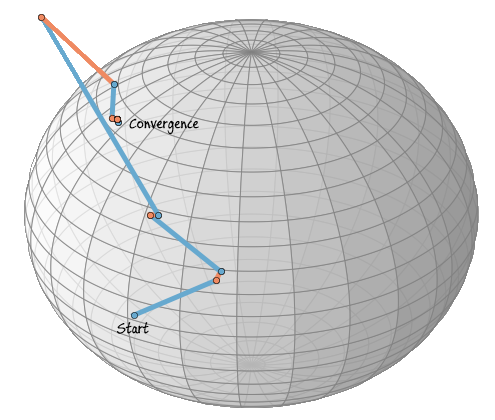
In this case the iteration has already converged after five steps, the following five steps are also plotted, but are stable and can’t be seen. The iteration converges when the Rayleigh quotient is minimized, therefore, we have now found an eigenvector to the randomly chosen matrix A.
Now we have everything we need to generate the figure above. First we define a couple of functions.
def RNmS(A, x0): # Iteration N = 5 xk = x0 for k in range(0, N + 1): Pxk = P(xk) M = (Pxk.dot(A).dot(Pxk) - f(A, xk) * I) y = -Pxk.dot(A).dot(xk) eta_k = linalg.solve(M, y) xk = R(xk, eta_k) X = A.dot(xk) / xk return X.mean() def find_nearest_index(array, value): index = ((array.real - value.real) ** 2 + \ (array.imag - value.imag) ** 2).argmin(0) return index
The we pick a matrix and calculate the eigenvalues with the standard algorithm for comparison.
# Choice of 3x3 symmetric matrix for which we want to find the eigenvectors/-values. # Note that different matrices produce very different images. A = random.randint(0, 10, (3, 3)) A = dot(A, A.T) EW, EV = linalg.eig(A) print "Eigenvalues: ", print EW
Finally we make a spherical grid, perform the iteration for every point in the grid, and plot the result.
# Resolution n = 512 nj = n * 1j # u and v are parametric variables. u = r_[0:2*pi:nj] v = r_[0:pi:nj] x = outer(cos(u), sin(v)) y = outer(sin(u), sin(v)) z = outer(ones(size(u)), cos(v)) # Figure out which eigenvectors/-values the algorithm converges to # for all the spherical initial vectors. s = zeros((n, n)) for i in range(0, n): for j in range(0, n): try: X = RNmS(A, array([x[i, j], y[i, j], z[i, j]])) s[i, j] = find_nearest_index(EW, X) except: raise print X print "Indexes: ", print set(s.flatten()) bmap = brewer2mpl.get_map('RdBu', 'Diverging', 3) cmap = bmap.get_mpl_colormap(N=3, gamma=1.0) figsize(50, 50) fig = plt.figure() ax = fig.add_subplot(111, projection='3d') ax.set_aspect('equal') ax.scatter(x, y, z, c=s, s=16, edgecolor='none', marker='s', cmap=cmap); ax.axis("off");
