The effect of Poisson zeros on OLS regression results
In a previous post I wrote about the Poisson distribution seeming like a good error model for scRNA-seq counts. This suggests using GLM with Poisson likelihood to analyse your data, as long as the offset due to count depth variation is taken into consideration.
An alternative strategy could be to transform the counts to roughly normal, and perform analysis in that setting. This is effectively what the vast majority of studies do for unsupervised analysis: counts are transformed, then PCA is used to find a low-dimensional representation for further analysis such as clustering.
What if we try to adjust for the count depth variation in a supervised setting assuming Gaussian noise?
A huge benefit of assuming Gaussian noise is that linear regression has an extremely efficient solution, usually referred to as OLS regression. A couple of years ago I made a simple Python package NaiveDE to perform OLS regression on gene expression matrices. I don't recommend anyone use it for final analysis, indeed I called it "Naive DE" because it is a baseline. Literally every other DE test will be better than it by design, in particular with regards to false positive P-values. (Well maybe not according to a recent study, the test in NaiveDE should be equivalent to the t-test.) It is nevertheless convenient during exploratory analysis to iterate through models
Alternative and null models are specified by Patsy formulas, and significance is calculated with a likelihood ratio test. A Bonferroni corrected version of the P-value is also reported.
For every gene g where we have a design matrix X and observed counts yg we look at
The weights α are calculated by OLS, and σ2 is reflected in the residual errors. For flexibility, intercept is optionally part of the design matrix.
Negative control data
In the negative control 10X dataset from Svensson et al 2017, the only variation in observed expression should (in theory) be due technical effects, in particular the count depth variation. Here we are using 2,000 cells with 24,000 genes. The most common variance stabilizing transformation of scRNA-seq data is log(Y+1), so we will investigate how this affects regression.
If the gene counts are scaled per cells, we would want
We set up a model where the design matrix X have the log total counts, and an intercept. Ideally the weights for the log counts should be found to be 1, and the intercept 0. Note that in practice we are always using log(yg+1).
%%time lr_results = NaiveDE.lr_tests(sample_info, np.log1p(counts.T), alt_model='~ np.log(total_count) + 1', null_model='~ 1')
CPU times: user 2.98 s, sys: 702 ms, total: 3.68 s
Wall time: 3.35 s
The test produces a table with weights from the alternative model, hypothesis test restults.
print(lr_results.sort_values('np.log(total_count)', ascending=False).head(25))
                Intercept  np.log(total_count)           pval           qval
gene
ENSG00000198938  -5.501025             1.080920  3.073563e-294  6.147125e-291
ENSG00000198727  -5.600405             1.041435  3.073563e-294  6.147125e-291
ERCC-00002       -2.999032             1.034389  3.073563e-294  6.147125e-291
ERCC-00136       -4.155633             1.017020  3.073563e-294  6.147125e-291
ERCC-00113       -4.297474             1.010625  3.073563e-294  6.147125e-291
ENSG00000198886  -5.615521             1.010178  2.134557e-266  4.269114e-263
ENSG00000198712  -5.144020             1.005586  3.341643e-168  6.683285e-165
ERCC-00096       -2.740023             0.989442  3.073563e-294  6.147125e-291
ENSG00000210082  -4.357098             0.988333  3.073563e-294  6.147125e-291
ERCC-00046       -3.727992             0.979269  3.073563e-294  6.147125e-291
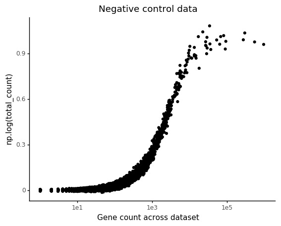
In this plot np.log(total_count) does not refer to the value, but weight for this variable. Each dot is a gene rather than droplet. The P-value comes from comparing the model with one that does not consider the depth.
The marjority of genes are found to have gene count weights much smaller than 1. It turns out that lowly abundant genes will have delfated total count slopes.
We can look at a few examples of genes with different count depth weights.
From this, it is clear that increased observations on the low count values, in particular 0, are responsible for decrease in the total count weight.
Differential expression
Now let us investigate how this count depth effect plays in to a differential expression analysis. With all published large scale experiments cataloging cell types, it is getting increasingly easy to simply fetch some data and do quick comparisons. We will use data from the recent single cell Mouse Cell Atlas30116-8). To get something easy to compare, we use the samples called "Brain" and focus on the cells annotated as "Microglia" and "Astrocyte". Out of the ~400,000 cells in the study, these two cell types have 338 and 199 representative cells. On average they have about 700 total UMI counts each, so while the entire study is a pretty large scale, the individual cell types and cells are on a relatively small scale. The final table has 537 cells and 21,979 genes.
print(sub_samples.head())
                            ClusterID Tissue    Batch        Cell Barcode  \
Cell name
Brain_1.AAAACGCGAGTAGAATTA   Brain_3  Brain  Brain_1  AAAACGCGAGTAGAATTA
Brain_1.AAAACGGAGGAGATTTGC   Brain_3  Brain  Brain_1  AAAACGGAGGAGATTTGC
Brain_1.AAAACGGGCTGCGACACT   Brain_2  Brain  Brain_1  AAAACGGGCTGCGACACT
Brain_1.AAAACGGTGGTAGCTCAA   Brain_3  Brain  Brain_1  AAAACGGTGGTAGCTCAA
Brain_1.AAAACGGTTGCCATACAG   Brain_3  Brain  Brain_1  AAAACGGTTGCCATACAG

                                    cell_type super_cell_type  is_astrocyte  \
Cell name
Brain_1.AAAACGCGAGTAGAATTA  Astrocyte_Mfe8 high       Astrocyte          True
Brain_1.AAAACGGAGGAGATTTGC  Astrocyte_Mfe8 high       Astrocyte          True
Brain_1.AAAACGGGCTGCGACACT            Microglia       Microglia         False
Brain_1.AAAACGGTGGTAGCTCAA  Astrocyte_Mfe8 high       Astrocyte          True
Brain_1.AAAACGGTTGCCATACAG  Astrocyte_Mfe8 high       Astrocyte          True

                            total_count  gene
Cell name
Brain_1.AAAACGCGAGTAGAATTA       1088.0     0
Brain_1.AAAACGGAGGAGATTTGC        967.0     0
Brain_1.AAAACGGGCTGCGACACT        543.0     0
Brain_1.AAAACGGTGGTAGCTCAA        679.0     0
Brain_1.AAAACGGTTGCCATACAG        957.0     0
In a differential expression test you simply include a covariate in the design matrix that informs the linear model about the different conditions you want to compare. Here we are comparing microglia and astrocytes.
%%time lr_results = NaiveDE.lr_tests(sub_samples, np.log1p(sub_counts.T), alt_model='C(is_astrocyte) + np.log(total_count) + 1', null_model='np.log(total_count) + 1')
CPU times: user 705 ms, sys: 136 ms, total: 841 ms
Wall time: 707 ms
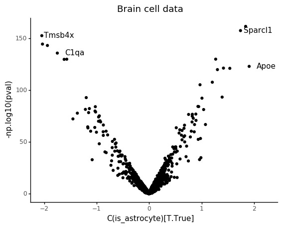
print(lr_results.sort_values('pval').head())
         Intercept  C(is_astrocyte)[T.True]  np.log(total_count)  \
Atp1a2   -1.925596                 1.840452             0.318532
Sparcl1  -1.008002                 1.742278             0.179123
Tmsb4x   -3.680027                -2.044908             0.948016
Hexb     -2.165802                -2.032087             0.646263
Ctss     -1.665139                -1.937761             0.553429

                pval           qval
Atp1a2   3.058918e-162  1.642639e-159
Sparcl1  3.548817e-158  1.905715e-155
Tmsb4x   2.742131e-153  1.472524e-150
Hexb     3.671724e-145  1.971716e-142
Ctss     8.167943e-144  4.386185e-141
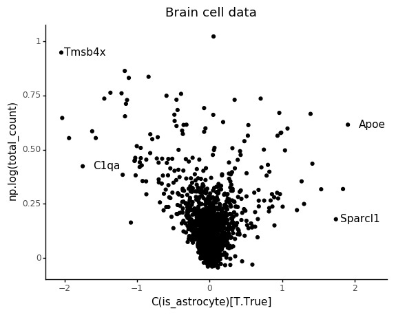
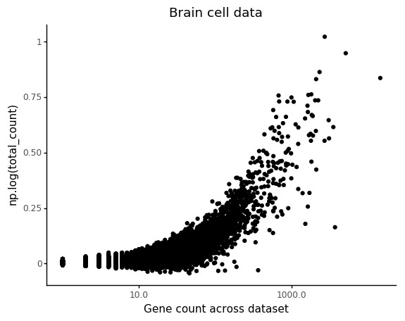
Also in this case we can see that the count depth weights are deflated for lowly abundant genes.
Similar to above, we can look at the relation between count depth and observed counts for a few genes, but we can also make sure to plot the stratifiction into the two cell types and how the regression models are predicting the counts.
Again we can see the overall abundance is related to the slope of the lines. Another thing which seem to pop out in these plots is an interaction between cell type and slope. For example looking at C1qa the slope for the microglia seem underestimated. This makes sense, if this is an effect of count noise at low abundances.
My takeaway from this is that OLS regression might be OK if counts are large, but at lower levels model parameters are not estimated correctly due to the count nature of the data.
Notebooks of the analysis in this post are available here.


