Illustrating spatially variable genes with a 1-dimensional zebrafish

The other day SpatialDE, our statistical test for spatially variable genes in spatial transcriptomics data was published in Nature Methods. The goal of the method is to find genes which in some way depend on the spatial organization of tissues, and for our paper we analysed generated with Spatial Transcriptomics, SeqFISH, and MERFISH. As a demonstration of how to use SpatialDE I also analysed some recent heart tissue. The underlying principle in SpatialDE can be hard to get to grips with, and the aim of this post is to provide an example that hopefully explains it.
One very practical reason it can be hard to see what is going on is that it is generally difficult to make plots to visualize data in more than 2 dimensions so that noise is easily interpreted. In terms of spatial gene expression, it is then easiest to make an example with a 1-dimensional tissue, and illustrate things that way.
There is actually a spatial transcriptomics dataset which is in fact 1-dimensional! In a study by Junker et al, the authors studied zebrafish embryos at the 15 somites stage by straightening them, then segmenting them into about 100 slices, each roughly 18 µm thick. For each slice digital RNA sequencing was performed providing expression levels for the entire transcriptome, annotated with the head-to-tail coordinates of the slice: a protocol they call “tomo-seq”. This provides an excellent example to illustrate what SpatialDE mean by “spatially variable genes”.

Defining spatial gene expression
Without pre-specifying the shapes of gene expression we need a way to express properties of how genes could behave across the coordinates. An effective way to look at this is to consider spatial coordinates as locally informative. If you know expression in a coordinate, then nearby coordinates should be pretty similar, while coordinates further away are still somewhat similar. In statistical terms, we say that coordinates \( x_i \) and \( x_j \) covary in a way that decreases with distance between \( x_i \) and \( x_j \). A common way to express this is through the Gaussian covariance function: \[ cov(x_i, x_j) = \exp \left(-\frac{|x_i − x_j|^2}{2 \cdot l^2}\right) \]
The parameter \( l \) describes the scale at which expression levels are locally similar. We illustrate the meaning of this by considering a length scale of 126 µm in the zebrafish embryo.

In this example, we don’t know what the expression values are in any coordinate, but we expect that expression levels 5 slices apart from each other will have a correlation of about 0.8, while expression levels 10 slices apart will have a correlation of about 0.4. In other words, genes may be expressed in or close to the head while not expressed at all in the tail, or vice versa. The right side of the plot shows a couple of expression curves drawn from a multivariate normal distribution with this covariance matrix.
\[ \begin{align*} y_g &\sim \mathcal{N}(0, \Sigma), \\ \Sigma_{i, j} &= cov(x_i, x_j) \end{align*} \]
Models like this where the covariance between points are parameterized are known as Gaussian processes.
Spatial and non-spatial variance
The curves above are random draws, but have you ever seen data that looks so clean? More likely there is additional noise which we cannot explain by only considering the spatial covariance between zebrafish slices. This can be expressed as \[ y_g \sim \mathcal{N}(0, \sigma^2 \cdot (\Sigma + \delta \cdot I)) \]
The \( \sigma^2 \) parameter is the overall magnitude of the variance of \( y_g \), while the \( \delta \) parameter scales how much of the variance not determined by spatial covariance. With these quantities (together with a correction for the structure of \( \Sigma \) called the Gower factor \( G(\Sigma) \)) we can move to a measure we refer to as “fraction spatial variance” (FSV), FSV \( = G(\Sigma) / (G(\Sigma) + \delta) \). This is a number between 0 and 1 which indicate how much of the variance in data is due to spatial covariance. To illustrate, we can randomly simulate data with different levels of FSV.
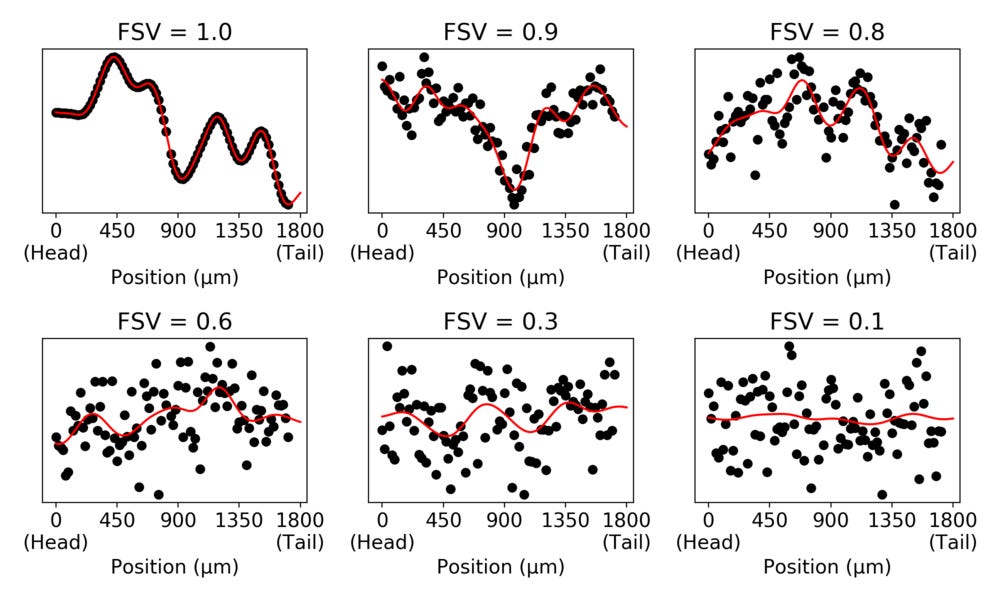
The simulated data in the panels have the same variance. But we can see that the spatial contribution to the variance decreases as the FSV decreases.
The SpatialDE test fits the \( \sigma^2 \) and \( \delta \) parameters to each genes observed expression levels, and also compares the likelihood with a model that has no spatial variance (FSV = 0) to obtain a significance level (p-value). This way it is possible to distinguish between genes with high variance and genes with high spatial variance. The \( l \) hyper-parameter for the \( \Sigma \) matrix is also fitted through grid search, so for each gene we also get the optimal length scale. (This dataset had 95 samples of 20,317 genes, and the SpatialDE test took about 5 minutes to run).
As an illustration, let us look at the expression patterns of a number of genes identified with different FSVs in the zebrafish embryo.

For the higher FSVs it is clear the expression depends on spatial location, while this is less clear for small FSVs. We can look at the relation between total variance and spatial variance, and how the FSVs are distributed compared to these.

On the right side the standard plot from SpatialDE illustrates the relation between the FSV and the statistical significance for all genes. I put in references to the genes I used as examples, as well as some genes that were highlighted by Junker et al in the original paper. In total SpatialDE identifies 1,010 genes as significantly spatially variable, with most of those genes having length scales between 65 µm and 244 µm.
Hopefully this one-dimensional example helps clear up what we mean by “spatially variable genes”, and also illustrate that there are many forms of data that can use spatial analysis. If you have spatial gene expression data, I recommend trying SpatialDE to identify genes of interest. The analysis associated with this post is available in a notebook here. If you want to use SpatialDE for your spatial data, you can install it by pip install spatialde. Thanks to Lynn Yi for editorial feedback on this post.