Training scVI - Posterior predictive distributions over epochs

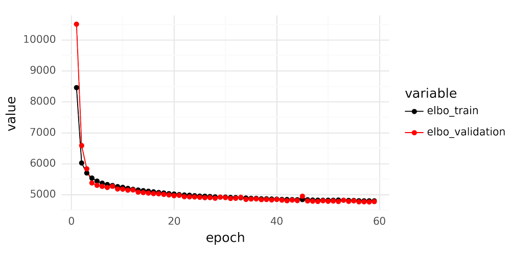
When fitting an scVI model for scRNA-seq data it is important to inspect the loss curves over epochs after finishing training. An example is shown below.

There are a couple of key features to look for when inspecting the loss curve. The validation loss should not dramatically deviate from the training set loss, as this indicates overfitting. A judgment call must also be made to determine whether to consider the training ‘finished,’ or if you should train for additional epochs. Once the loss plateaus, further training epochs yield no improvement. However, when is the curve ‘flat enough’ to be satisfactory?

The scVI model is formulated as:

$$ \begin{align*} z_n &\sim \text{N}(\mathbf{0}, I), \\ \rho_n &= f(z_n, s_n), \\ y_n &\sim \text{NB}(\rho_n \cdot \ell_n, \phi). \end{align*} $$

In the loss curves, model performance, representing estimation of gene expression for all cells and all genes in the data, is summarized by a single number. The loss reported during scVI training is the evidence lower bound (\( \text{ELBO} \)), defined as \( \text{ELBO} = \log p(y | z) - \text{KL}(q_\phi (z) || p(z)) \).

For smaller models, like univariate linear regression models represented as \( y \sim \text{N}(a \cdot x + b, \sigma) \), beyond looking at a single performance metric, it is beneficial to explore the posterior predictive distribution in relation to the observed data. In this linear regression example, the parameters \( a \), \( b \), and \( \sigma \) have the joint posterior distribution \( p( a, b, \sigma \ | \ x, y) \). The posterior predictive distribution describes the distribution of potential observations \( \tilde{y} \) given the seen observations \( y \) and the model, represented as $$ p(\tilde{y} \ | x, y) = \int_{a, b, \sigma} p(\tilde{y} \ | \ a, b, \sigma) p(a, b, \sigma \ | \ x, y) d (a, b, \sigma). $$

Analyzing a posterior predictive distribution allows a user to understand potential variation in the data that the model might overlook, or determine the breadth of the posterior predictive distribution.

With Bayesian models, examining the posterior predictive distribution requires sampling from the posterior distribution of the parameters, integrating these parameters into the likelihood distribution, and then drawing samples from the combined distribution. For the scVI model, the procedure is:

$$ \begin{align} \tilde{Z} &\sim p(Z | Y), \\ \tilde{\rho} &= f(\tilde{Z}, s), \\ \tilde{Y} &\sim \text{NB}(\tilde{\rho} \cdot \ell, \phi). \end{align} $$

As an illustrative example of looking at posterior predictive distributions from an scVI model, an scRNA-seq dataset from (Zhu et al. 2023) is chosen. The full dataset comprises 139,761 blood cells with measurements for 33,528 genes from 17 human donors. For illustrative purposes a random sample of 20,000 cells from this dataset is selected, ensuring each epoch provides 20,000 examples to the model (using the entire dataset leads to rapid convergence, making it challenging to observe the training effect).

Reviewing the posterior predictive distribution for an scVI model involves examining distribution densities for tens of thousands of genes across tens of thousands of cells. To obtain a general understanding of the posterior predictive distribution, a smaller subset of cells and genes is chosen, and the posterior posterior predictive distributions for this subset are analyzed.

By employing this limited set of cells and genes, it is possible to sample from the posterior predictive distribution after each training epoch. This process allows for an understanding of how decreases in the model’s loss function correlate with its ability to emulate training data.

The animation below shows UMI count histograms of 128 samples from the posterior predictive distributions of an scVI model as black bars for five cells and 10 genes across 60 epochs of training. The red bar marks the observed UMI count for each cell-gene combination.

View fullsize

After the first epoch, most samples from the posterior predictive samples are zeros or show very low counts compared to the observed counts indicated by the red lines. Following the second epoch, the posterior predictive distribution undergoes a significant shift, producing very broad count ranges for each cell-gene combination. In subsequent epochs, the posterior predictive distributions become more focused and align closer with the observed counts. Histograms of posterior predictive distribution counts for observations of zero shrink to mostly generate zeros.

Beyond the 40th epoch, the posterior predictive distributions remain largely unchanged. By the 60th epoch, all observed counts for this cell-gene subset overlap with samples from the posterior predictive distributions.

Jupyter notebooks for generating posterior predictive distributions are available on GitHub.