Extract Cluster Elements by Color in Python Dendrograms

One aspect of using Python for data analysis is that hierarchical clustering dendrograms are rather cumbersome to work with. Both in terms of plotting next to a heatmap, and how to relate the input data to the resulting plot. Ideally the dendrogram function would return a proper instances of some Dendrogram class. But let’s work with what we have.

There are plenty (1, 2) of guides around on how to make R inspired heatmaps with dendrograms. Here I will describe how to parse out the cluster members as seen in a dendrogram, which can be handy if one notices interesting patterns in the corresponding heatmap.

Let’s start with importing some modules.

%pylab inline

from collections import defaultdict

import pandas as pd
from scipy.cluster.hierarchy import dendrogram, set_link_color_palette
from fastcluster import linkage
import seaborn as sns
from matplotlib.colors import rgb2hex, colorConverter

numpy.random.seed(0025)

We also set some prettier non-default colours.

sns.set_palette('Set1', 10, 0.65)
palette = sns.color_palette()
set_link_color_palette(map(rgb2hex, palette))
sns.set_style('white')

We should create some simple example data for the purpose of illustration.

x, y = 3, 10
df = pd.DataFrame(np.random.randn(x, y),
                  index=['sample_{}'.format(i) for i in range(1, x + 1)],
                  columns=['gene_{}'.format(i) for i in range(1, y + 1)])

link = linkage(df, metric='correlation', method='ward')

figsize(8, 3)
den = dendrogram(link, labels=df.index, abv_threshold_color='#AAAAAA')
plt.xticks(rotation=90)
no_spine = {'left': True, 'bottom': True, 'right': True, 'top': True}
sns.despine(**no_spine);

The dendrogram function will return a dictonary containing a representation of the tree as plotted.

den

{'color_list': ['#c13d3f', '#AAAAAA'],
 'dcoord': [[0.0, 0.70210454159043401, 0.70210454159043401, 0.0],
  [0.0, 1.1003608323279817, 1.1003608323279817, 0.70210454159043401]],
 'icoord': [[15.0, 15.0, 25.0, 25.0], [5.0, 5.0, 20.0, 20.0]],
 'ivl': ['sample_3', 'sample_1', 'sample_2'],
 'leaves': [2, 0, 1]}

The tree is represented as a collection of ∏ shaped components.

The three items named color_list, dcoord, icoord indexes these ∏’s

Obviosly color_list contains the colors. The lists in dcoord contain the y coordinates of the ∏’s (the distances) while icoord has the x coordinates. These would be the index coordinates.

In the minimal example above we have two ∏’s, and one can see that the x-coordinates are repeated once.

The coordinates go from left to right. So for the red ∏, the ‘legs’ are located at 15 and 25, while the grey one has legs at 5 and 20.

The apperant pattern is that legs positioned at leaves will end with 5. The reason is to nicely place the leg at the middle of the corresponding leaf index value. This also implies the actual list indices of the leaf are multiplied by 10.

Thus we first subtract 5 from each colors icoord, then divide by 10. If the resulting number is close to the closest integer, we consider this to be an index for a leaf. If the resulting number is not close to an integer index, it means the colored tree we got it from is from non-leaf parts of the trees.

For each leaf, we add it to a list per color in a dictionary.

cluster_idxs = defaultdict(list)
for c, pi in zip(den['color_list'], den['icoord']):
    for leg in pi[1:3]:
        i = (leg - 5.0) / 10.0
        if abs(i - int(i)) < 1e-5:
            cluster_idxs[c].append(int(i))

cluster_idxs

defaultdict(<type 'list'>, {'#c13d3f': [1, 2], '#AAAAAA': [0]})

Next we need to grab the labels of the leaves given the indexes. But before we do that, since it’s difficult to keep track of what color e.g. #c13d3f is, we make make an IPython notebook compatible HTML representation of the dictionary holding the information. Objects of this class will behave just like dictionaries, except for representing them as a HTML table.

class Clusters(dict):
    def _repr_html_(self):
        html = '<table style="border: 0;">'
        for c in self:
            hx = rgb2hex(colorConverter.to_rgb(c))
            html += '<tr style="border: 0;">' \
            '<td style="background-color: {0}; ' \
                       'border: 0;">' \
            '<code style="background-color: {0};">'.format(hx)
            html += c + '</code></td>'
            html += '<td style="border: 0"><code>' 
            html += repr(self[c]) + '</code>'
            html += '</td></tr>'

        html += '</table>'

        return html

(Note that the representation uses colerConverter from matplotlib, so it supports any matplotlib supported color representation, not only hex color strings.)

Now just go through the list of indices and fetch labels.

cluster_classes = Clusters()
for c, l in cluster_idxs.items():
    i_l = [den['ivl'][i] for i in l]
    cluster_classes[c] = i_l

cluster_classes

#c13d3f	['sample_1', 'sample_2']
#AAAAAA	['sample_3']

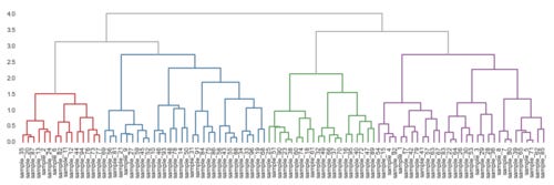
Let’s combine this to a nice reusable function, and try it out on a larger example.

def get_cluster_classes(den, label='ivl'):
    cluster_idxs = defaultdict(list)
    for c, pi in zip(den['color_list'], den['icoord']):
        for leg in pi[1:3]:
            i = (leg - 5.0) / 10.0
            if abs(i - int(i)) < 1e-5:
                cluster_idxs[c].append(int(i))

    cluster_classes = Clusters()
    for c, l in cluster_idxs.items():
        i_l = [den[label][i] for i in l]
        cluster_classes[c] = i_l

    return cluster_classes

x, y = 96, 10
df = pd.DataFrame(np.random.randn(x, y),
                  index=['sample_{}'.format(i) for i in range(1, x + 1)],
                  columns=['gene_{}'.format(i) for i in range(1, y + 1)])

link = linkage(df, metric='correlation', method='ward')

figsize(12, 4)
den = dendrogram(link, labels=df.index, abv_threshold_color='#AAAAAA')
plt.xticks(rotation=90)
sns.despine(**no_spine);

get_cluster_classes(den)

#c13d3f	['sample_20', 'sample_87', 'sample_35', 'sample_2', 'sample_24', 'sample_13', 'sample_6', 'sample_82', 'sample_11', 'sample_12', 'sample_44', 'sample_94', 'sample_73', 'sample_77', 'sample_76']
#4e7ca1	['sample_56', 'sample_81', 'sample_69', 'sample_9', 'sample_27', 'sample_21', 'sample_45', 'sample_52', 'sample_59', 'sample_46', 'sample_93', 'sample_10', 'sample_48', 'sample_78', 'sample_14', 'sample_50', 'sample_31', 'sample_91', 'sample_75', 'sample_86', 'sample_84', 'sample_55', 'sample_88', 'sample_43', 'sample_58', 'sample_33', 'sample_96', 'sample_34', 'sample_19', 'sample_68', 'sample_21']
#8e5d93	['sample_4', 'sample_92', 'sample_15', 'sample_54', 'sample_1', 'sample_17', 'sample_42', 'sample_79', 'sample_41', 'sample_57', 'sample_63', 'sample_67', 'sample_22', 'sample_64', 'sample_83', 'sample_30', 'sample_53', 'sample_26', 'sample_3', 'sample_29', 'sample_28', 'sample_36', 'sample_7', 'sample_80', 'sample_8', 'sample_5', 'sample_71', 'sample_65', 'sample_39', 'sample_62', 'sample_85']
#5e9d5c	['sample_23', 'sample_38', 'sample_90', 'sample_51', 'sample_25', 'sample_60', 'sample_74', 'sample_18', 'sample_61', 'sample_32', 'sample_49', 'sample_37', 'sample_70', 'sample_66', 'sample_16', 'sample_95', 'sample_40', 'sample_72', 'sample_47', 'sample_89', 'sample_40']

There is also an IPython notebook version of this post here