Integrating scRNA-seq and spatial STARmap data from mouse frontal cortex with scVI
In the last few months a number of interesting brain single cell datasets have been published. The new promising STARmap method was pusblished by Wang et al in Science using mouse brain data as example applications. Even more recently, two back to back mouse brain atlases were published in Cell. Zeisel et al characeterized the nervous system of adolescent mice through sequencing over 500,000 cells from 19 different regions using the 10X Genomics Chromium technology. Saunders et al studied adult mouse brain using almost 700,000 cells from 9 regions of the brain using the Drop-seq method.
All three papers contain some data from the frontal cortex region. An interesting exercise is to see how these datasets relate to one another, and if they can be analysed as a single entity.
The Wang et al STARmap data measures a panel of 166 genes in the medial prefrontal cortex (mPFC), across 3,700 cells from three separate biological samples. The STARmap data does not have any clusters annotated, but they do have spatial locations in the tissue preserved! The data from Saunders et al and Zeisel et al are transcriptome wide, so much larger. But it would be interesting to see how well the small panel of STARmap genes would work to integrate and analyse these datasets.
The anterior cortex data from Zeisel et al consists of 14,000 cells with annotations for 53 clusters (though some of these seem to be enteric neurons which is a bit odd?). The frontal cortex dataset from Saunders et al has over 70,000 cells annotated with 62 clusters. For the sake of simplicity, here I randomly sampled 15,000 cells from the Saunders data.
When the datasets are combined we get an expression matrix with 32,000 cells with counts in 158 genes. To analyze the data together I use scVI an autoencoder based method that have been working well in my current research work. Technology specific effects can be accounted for by providing them as batches.
Because we are looking at very few genes here, running inference on the scVI model takes about 10 minutes for 100 epochs. The scVI model then gives you access to a low-dimensional (10 dimensional in this case) latent representation space which can be used to generate counts for all genes consistent with the structure in the original data. The main point with this is that many machine learning and statistical methods that have problems with count data
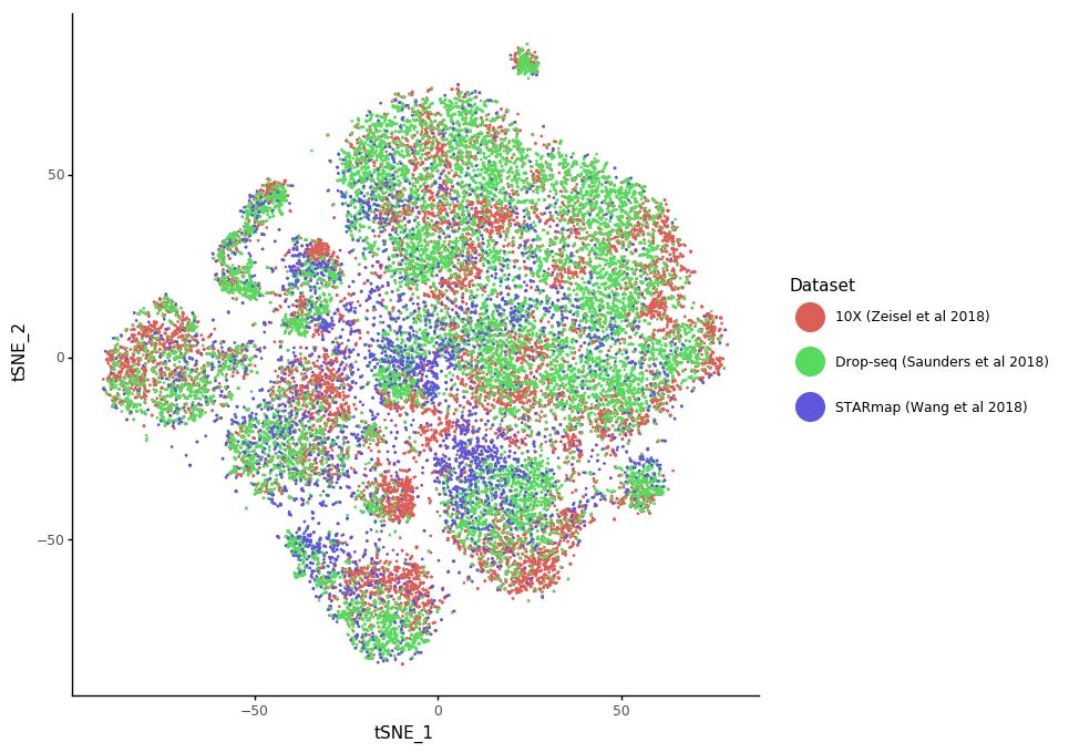
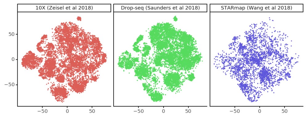
Once the scVI model is fitted, it is a good idea to create a tSNE of the latent space, and color the cells by various known factors to try to figure out what might contribute to variation in the data.
We see that similar patterns of densities overlap for all the datasets. Of course we need to remind ourselves not to read too much into the tSNE representation; the important part is the 10-dimensional latent representation of the data.
We can note that on the larger annotated scale annotation from the Zeisel and Saunders we can see overlap between related terms in the tSNE! Immune cells close to immune cells, neurons close to neurons, etc.
We can also color the cells by the complete cluster annoation. But with so many clusters it becomes hard to tell the colors apart! (And here I even collapsed some of the Saunders et al cluster names so they would fit in the plot.)
To learn about how the different annotations in the different datasets relate to each other we can use Ward linkage on the cell group centers to create a common dendrogram for all the groups. Because of the design of the latent space, we can simply use Euclidean distances. First we look at the broad cell classes from both the annotated datasets.
From the dendrogram it is clear that the class annotations are consistent between the datasets, as we observed in tSNE above.
We turn then to looking at all 110 annotated clusters in the frontal cortex data from the two publications. This dendrogram is on the larger side, bu the text is stil legible. While it seems pretty consistant within a given dataset, the mixing does not seem completely right. For example neurons in the Saunders et al data are mixed with oligodendrocytes from the Zeisel et l data. This is not necessarily terrible, we are only working with 158 genes from the STARmap panel, the original studies used thousands of genes to define the cell types.
The STARmap cells do not come with cell type annoations. They do however come with spatial locations for every cell! We can try to link the spatial locations in the STARmap data with the cell type annotion in the othe data sets.
scVI has specialized functionality for these tasks, both for semi-supervised learning to annotate cells, and for working with combined spatial and scRNA-seq datasets. Here however we will just do something simple to see how it works out.
Since Euclidean distances are meaningful in the latent 10-d space, we can use a kNN classifier using clusters or classes as targets.
Now we can plot the spatial locations of the STARmap cells, but annotate the cells with predicted clusters from the scRNA-seq datasets. This way we can qualitatively evaluate whether the clusters are consistent with spatial structure in the brain.
In these plots above, each "stripe" consists of different biological samples, and it wouldn't make sense to plot the cells from different biological samples in a single plane. I think they are even from different mice.
From this it seems that prediction to the annotation from Saunders et al seem more spatially organized in the STARmap data.
The cell types in the Zeisel et al data are predicted more spread out in the STARmap data. I suspect there is an issue with the cell type annotation here, since excitatory neurons (TEGLU*) are mapped to the region at the right which is supposed to be non-neuronal. I might have misunderstood how the cell clusters are indexed in the Loom files for cortex. (There is also an odd thing where the website says there are 7,000 anterior cortex cells, but the Loom file contains 15,000).
A notebook with all analysis, including fitting the scVI model, is available here.


