Variance stabilizing scRNA-seq counts — What do you mean "heterogeneity"?

Quantitative sequencing assays in general yield counts. The generative models for different levels of counts are in many ways fundamentally different from continuous distributions such as the more common Gaussian (normal) distribution. The problem is not that the data consists of integers; rounded normal data such as e.g. user ratings of products wouldn't have any particular problems being analysed with normal methods. Counts however are generated by several, cumulative, singular events. With each of the events having some probability of occurring in a given "time interval" or other relevant unit.

For example, if we think about the RNA sequencing process in the abstract we have a large collection of cDNA molecules which are randomly sampled and identified as originating from genes. How often moleculas are identifed from any particular gene tells us something about the abundance or expression level of the gene. The process of counting however implies that variation will propagate as the number of events increase. The effect of this is that there will be an inherent relation between mean (expected value) and variance of counts.

As an example, let us look at two recent datasets. One from Karaiskos et al where the authors mapped out fruit fly development on the single cell level, and another from Stoeckius et al where the authors developed a new method to study RNA and protein expression from cells in tandem.

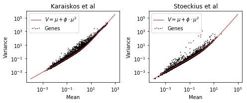
The mean-variance relation typical for negative binomial distributed count data is quite clear. Negative binomial, or other similar distributions, have been used to study RNA-seq data for a long time. Almost all statistical tests for comparing control vs condition style experiments (differential expression) use generalized linear models assuming count data with these kinds of distributions.

Single cell RNA-seq data is different. Not necessarily because the data wouldn't be suitible for these tools, but rather because differential expression is a minor question of limited interest in single cell studies. By far the most popular use of scRNA-sequencing is to identify groups of cells which are similar to eachother and might correspond to functionally distinct cell types. In addition to such clustering analysis, inference of developmental trajectories are popular, as well as quantifying the degree of variation between conditions.

So unlike bulk RNA-sequencing, the key analysis modality is in terms of multivariate analysis such as clustering or "dimensionality reduction" like PCA. In the coming years I believe figuring out effective ways to think about these issues for count data will be important, especially for sparse counts from low depth!

In the meantime, it is useful to be able to use available methods. Existing methods for clustering or dimensionality reduction are almost always either explicitly or implicitly designed with normal data in mind. (A notable exception being ZINB-WaVE by Risso et al). Any method using Euclidean distances implies normally distributed data.

One way to deal with these problems is to transform the data) in some way which makes it more similar to normal data. The logarithm is a very practical transformation for positive data. In particular ratios are very useful to log transform. With counts though, it is common to observe values of zero, for which the logarithm is not defined. Instead, it is common to perform \( \log(x + 1) \) for counts \( x \).

If we apply this transformation to each gene \( i \), we can investigate a couple of things. First of all, we can see what happens with the mean-variance relation. Secondly, we can display the first few principal components for both of the data sets using the transformed unit. This will represent a form of multivariate analysis.

From the plots we can observe a few things. For higher mean counts the relation between mean and variance (or standard deviation) is gone. However, for lower counts (mean \( < 1 \)) there is still some correlation. From the PCA below we can see some subpopulations for each data set.

The 1 here was added due to the observed zero counts. But why 1? What if we used something else? Is this the best we can do? In the end, adding the one was quite ad hoc wasn't it? Or in the words of Arjun Raj the other week:

Am I the only one who finds this log(x+1) thing everyone does all the time incredibly inelegant?
— Arjun Raj (@arjunrajlab) September 28, 2017

There is actually some theory we can use here. Our goal was to transform the data in way that removes the mean-variance relation as effectively as possible. This is known as a variance-stabilizing transformation. For example, in bulk RNA-sequencing the DESeq2 package has a function vst() for this (based on the underlying parametric Poisson-Gamma model).

If there is a functional form for the relation between the mean and the variance, e.g.

\[ Var(x) = g(\mu), \]

then the variance can be stabilized by applying the function

\[ f(x) = \int^x \frac{1}{\sqrt{g(v)}}dv. \]

As illustrated in the first plot of the post, for negative binomial data, which generally suits scRNA-seq counts well, we have that

\[ Var(x) = \mu + \phi \cdot \mu^2, \]

where \( \phi \) is the dispersion for the data. If we plug this into the integral above, and use Wolfram Alpha to solve the integral because I'm not in school anymore, we get

\[ VST(x, \phi) = 2 \cdot \frac{\sinh^{-1} \left( \sqrt{ \phi \cdot x } \right)}{\sqrt{\phi}} \]

It is very easy to find a \( \phi \) for the data by fitting a polynomial to the observed mean-variance relation. Let's transform our data in this way, and redo the plots for the two data sets.

We can note that this transformation behaves very similarly to \( \log(x + 1) \). One difference is that the standard deviation is scaled around 1 rather than around 0.5. Any effect on the PCA seems minimal though.

In a 1948 paper Anscombe explored these sorts of tranformations for Poisson and negative binomial data. In addition to the \( \sinh^{-1} \) form of the solution to the integral, Anscombe also considers an approximation which works for certain ranges of mean and \( \phi \). The approximation has the form \[ \log\left( x_i + \frac{1}{2 \cdot \phi} \right). \]

This has the same form as the heuristic \( \log \) transform, but instead of just picking 1 the "pseudocount" is motivated by the data distribution and statistical theory. We also create the same plots as above for data tansformed in this way.

Again the data looks similar to before, and we're back to the situation of having standard deviation around 0.5 for highly expressed genes.

In both of these cases we have assumed a global \( \phi \) parameter, and found it by polynomial curve fitting of mean vs variance. This is handy because we can use information from all genes and learn something global about the data. Then each gene is transformed assuming a fixed dispersion level.

For these data sets, there's actually no real need to assume a global \( \phi \). They have thousands of cells providing observations for each gene, we can easily learn individual \( \phi_i \) for each gene by maximum likelihood. That means we can perform VST of each gene independent of the other genes.

(It should be mentioned that finding all the \( \phi_i \)'s took about 40 minutes for the larger of the data sets, so it's not extremely practical).

When plotting these independent VST values we first see that the relation between mean and standard deviation is much "tighter" for both data sets. We still get an interesting bump for lower expression values, but after a mean of 2.0 the standard deviations are stable at 1.0. (A problem of course is that it's hard to know what "2.0 expression" means here, but it seems somewhat comparable between the two data sets).

Here we notice that the low-dimensional representation in the PCA is different from the previous data transformations. For the left data, we don't see clear clusters anymore, while for the right data some within-cluster covariance seem to follow PC1 better.

Finally, we can try to perform the approximate Anscombe transformation for gene specific \( \phi_i \) values.

It's hard to say what we are seeing here. There's definitaly no apparant correlation between mean and variance after the transformation. Though the standard deviations are not particularly stable around a value. For very high mean expression, values are transformed to have 0 standard deviation, meaning they are probably transformed to a constant value.

The multivariate PC analysis shows similar results as the first few transformations.

In the end I don't have any particularly good conclusions. The results are in the end somewhat different, especially when considering per gene \( \phi_i \) values. I have no idea which would "correct" in any meaningful way.

One note though, is that in all cases (except the last) there still is a dependency between mean and variance for genes with very low means. Considering that scRNA-seq as a field is moving towards more cells rather than more counts per cell, this might mean that variance stabilizing transforms are the wrong way to go in modern studies. Instead working directly with count distributions might be a more stable strategy for low counts. There of course is very limited prior work on this, and that is good to keep in mind when working with and planning to make shallow scRNA-seq data.