Count depth variation makes Poisson scRNA-seq data Negative Binomial

In the scRNA-seq community the observation of more zero values than expected (called the "dropout problem") is still a concern. The source seems to be an intuition that at such small scales of biological material as RNA from individual cells, molecular reactions lose efficiency due to conceptual stochastic events. The trendiest computational research directions in the field at the moment are probably tied between "how do we do this for a million cells?" and "how do we deal with the dropouts?". In particular droplet based scRNA-seq methods are considered to have more dropouts, often leading investigators that opt for more expensive plate based methods even for exploratory pilot experiments.

In negative control data there is no evidence for zero inflation on top of negative binomial noise, counter to what is commonly suggested (in particular for droplet based methods). A notion that has inspired significant research efforts. A recent interesting report by Wagner, Yan, & Yanai goes even further and illustrates that the Poisson distribution is sufficient to represent technical noise in scRNA-seq data. The authors write that additional variation in gene counts is due to efficiency noise (an observatin from Grün, Kester, & van Oudenaarden that different tubes of reagents appear to have different success rates), and can be accounted for by an averaging approach.

This can be explored by simulating data! Say droplets contain transcripts from 300 genes, whose relative abundance levels are fixed because they come from the same RNA solution. Then a droplet with \( d \) transcripts can be seen as a draw from a multinomial distribution,

\[ c_i \sim \text{Multinom} (d, (p_1, \ldots, p_{300})). \]

Now each gene will independently conform to a Poisson distribution.

The constant mean-variance relation for Poisson holds (as expected) for this simulation. In actual data, genes with higher abundance are over dispersed, which can be modeled using a negative binomial distribution.

The negative binomial distribution is constructed as a mixture of Poisson distributions, where the rate parameter follows a Gamma distribution. Other Poisson mixtures have also been suggested for scRNA-seq data.

An aspect of real data which our mutlinomial simulation does not account for is that the total counts observed in each droplet is variable. Indeed, usually a cutoff at some low number of total counts per droplet is used to decide which droplets captured cells and which only contain background material that is not of interest.

Thinking about the abundance levels of the different genes as rates in Poisson distributions require each observation to come from a constant count depth. If the count depth varies in each observation but the model is not informed of this, it will appear as if the rate for each gene is variable, and this will be more consistent with a negative binomial distribution.

As an illustration, in the simulation, variation in count depths can be included. For simplicity, a uniform distribution is used,

\begin{align} d_i & \sim \text{Uniform}(5.000, 100.000), \\ c_i & \sim \text{Multinom} (d_i, (p_1, \ldots, p_{300})). \end{align}

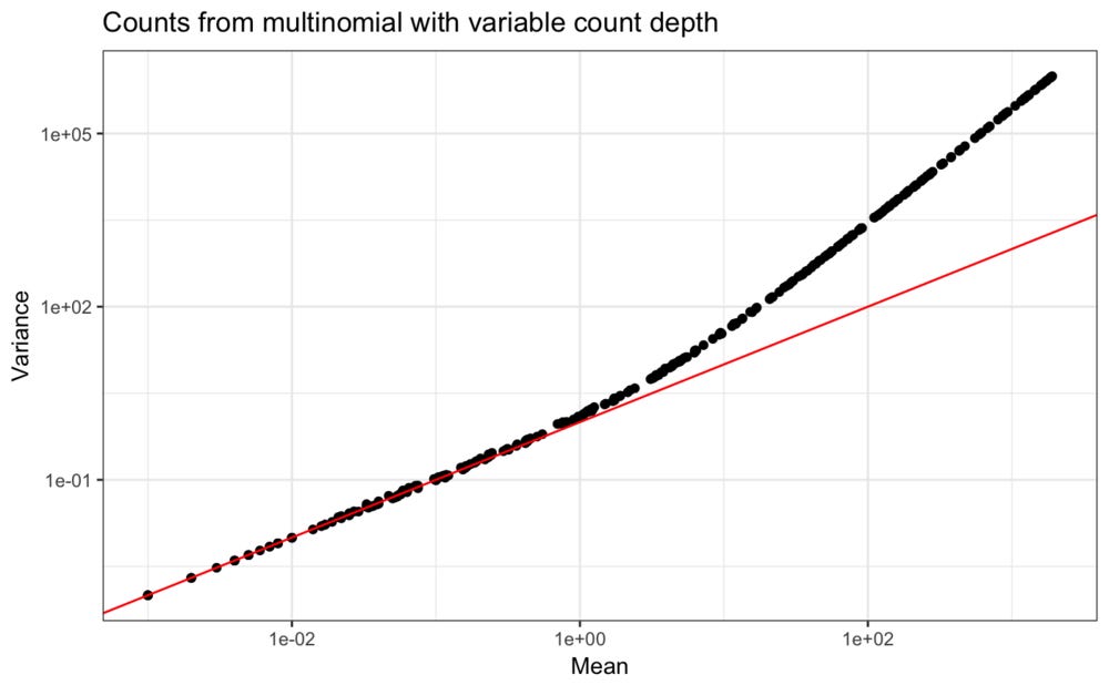
These new values clearly have the quadratic polynomial mean-variance relation that is typical for scRNA-seq counts.

This indicates we need to handle the differences in count depth. The easiest solution is to simply divide the expression counts in each cell with the total depth, turning each expression value into a fraction.

In the RNA-seq field it is also common to also multiply these fractions by 1 million to form the "CPM" unit.

It is clear that after creating either fractions or CPM will follow a linear relation between mean and variance. However, in both cases there is an offset from the unit relation, and in particular for the CPM unit the variance gets inflated compared to the mean.

The thrid panel shows the result after manually scaling the fractions (through multiplication by 3.5e4) to achieve the Poisson mean = variance relation. (There is probably a closed form expression for the scaling factor that achieves this, and the 1e6 is above this, explaining the variance inflation.)

It is entirely possible that the this type of scaling to create CPM from fractions is one reason people have noticed higher than expected numbers of zeros. For Poisson data, the expected number of zeros at a given mean expression level is given by the function \( e^{-\mu} \).

The counts themselves follow the theoretical curve quite close, but with an increase of zeros at high expression levels, consistent with negative binomial zeros. 'Fractions' see a large offset of much fewer zeros than is expected given the mean, while CPM see an offset for more zeros than expected. The manually scaled values follow the theoretical curve decently, though far from exactly.

For interpretable analysis, counts should be scaled for total count depth, but this also need to be taken under consideration when looking at the results (e.g. dropout rate). The best solution might be to take inspiration from the field of generalised linear models. In that field offsets are included in models when there is a clear explanation for variation in counts, to convert counts to rates. Clustering or pseudotime methods could be reformulated to the Poisson setting with offsets.

There are some additional aspects to keep in mind. For negative control data where each droplet contains RNA from the same solution, the count depth variability must be technical, but in real samples this could also be due to cells having variable amounts of RNA. For droplet based data one simple reason for the heterogeneity could be due to variation in coverage for DNA oligos on barcoded beads. It is not clear what an explanation for plate based methods would be, and no proper negative control data exist for plate based methods to investigate these properties. On a similar note, the latest single cell sequencing methods based on stochastic schemes for in situ barcoding of cells are impossible to assess with negative control samples.

An R notebook for this analysis is available here. Thanks to Lior Pachter for editorial feedback on this post.