Improper applications of Principal Component Analysis on multimodal data

When reading papers I have noticed some strange PCA plots. An example of this I stumbled over today was this one, Figure 1B from Kim et al., 2015, Cell Stem Cell 16, 88–101.

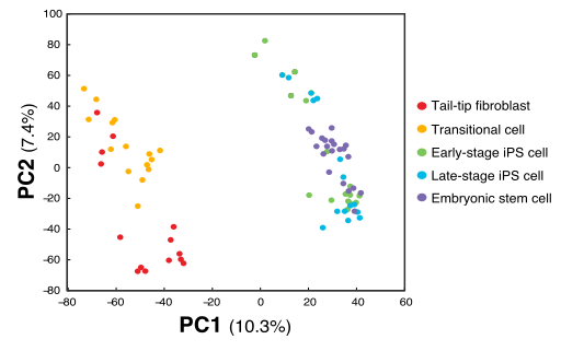
The odd thing here is that there are two obvious subpopulations of points, but within each they appear to have the same slope of PC1 vs PC2. This indicates that there is a linear dependence between PC1 and PC2, with some other factor explaining the difference between the clusters. In the case of the paper they only make this plot as a way to illustrate the relation between the samples. But if there where to be any additional analysis of the components in this PCA, this relation between PC1 and PC2 tells us something is wrong.

I made an artificial example to highlight this issue using Python.

from sklearn.preprocessing import scale
np.random.seed(8249)

N = 500
mode = np.random.randint(0, 3, N) * 10

x = np.random.normal(0, 100, N)
y = mode + np.random.normal(0, 1, N)

X = np.vstack([x, y]).T
X = scale(X)

figsize(6, 6)

plt.scatter(X.T[0], X.T[1], c='k', edgecolor='w', s=50);
sns.axlabel('x', 'y');

plt.title('Generated data');

This data is 2-dimensional with one normally distributed variable accounting for the x-axis, and the y-axis being due to membership in one of three discrete classes, with some normally distributed noise added. Imagine that we don’t have the information about the two processes generating the points, and we wish to find a model for the points by latent factors. We apply principal component analysis to this data.

from sklearn.decomposition import PCA

pca = PCA()
Y = pca.fit_transform(X.copy())

figsize(6, 6)

plt.scatter(Y.T[0], Y.T[1], c='k', edgecolor='w', s=50);

sns.axlabel('Principal Component 1', 'Principal Component 2');

plt.title('Principal Component Analysis');

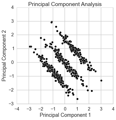
The issue is that principal component analysis seeks to primarilly find a projection of the data to one dimension which maximizes the variance. If your data is multivariately normally distributed the PCA will find the “longest” factor explaining the data. But this does not hold when the data one is working with is for example multimodal. Like in this trimodal case. The largest variance is obviosly over the diagonal of the square-like area spanned by the points. But for finding a latent factor model with this kind of data variance is simply not so useful as a measure.

In this case it might make sense to use Independent Component Analysis (ICA) in stead. It is a strategy for finding latent factors which aims to make the latent factors searched for as statistically independent as possible. It makes no assumption about the distribution of the data.

from sklearn.decomposition import FastICA

ica = FastICA()
Z = ica.fit_transform(Y.copy())

figsize(6, 6)

plt.scatter(Z.T[0], Z.T[1], c='k', edgecolor='w', s=50);
sns.axlabel('Independent Component 1', 'Independent Component 2');
plt.title('Independent Component Analysis');

One immidate caveat with ICA over PCA is that there is no longer an ordering of the components, component 1 does not necesarilly explain more of the variability of the data than component 2. They are both equally important for the inferred latent variable model.

It is clear here though that component 1 corresponds to the membership, and component 2 to the x-variable.

If you are expecting clusters in your data, PCA is probably not the right tool.