Timecourse analysis with Sleuth — What do you mean "heterogeneity"?

An extremely interesting application of RNA-sequencing analysis is to study samples over a time series. This allows you to identify patterns of expression over some response to a stimuli or developmental progression.

While Sleuth together with the Kallisto from the Pachter lab makes it easy to perform differential expression analysis in the two-condition case of an RNA-seq experiment, there is still some confusion about how to perform DE over a time series. I thought it would be useful to write an example text of how to detect DE transcripts over a time course with Sleuth.

The first problem is to define what we mean by differentially expressed in the context of a time series. For a treatment-vs-control type experiment it is simple: What genes are higher or lower expressed in the treatment condition compared to the control? The first generalization which comes to mind would be to find genes whose level increase or decrease with the time points. This means finding correlation with time points and boils down to linear regression of expression with time points. However, this will mask potentially interesting genes which could for example peak in the middle of the time series. What we want is to find if the expression of a gene follows a general pattern to a higher degree than just noise.

In a linear modelling framework, such as Sleuth, a common solution for this is to use natural splines. Given a number of degrees of freedom for a natural spline model, knots will be placed along the quantiles of the observations of the time axis, which will define basis polynomials with local support.

$$ Expression \sim \beta_0 + \sum_{i=1}^3 \beta_i B_{i}(Timepoint) + \varepsilon $$

The idea is now to compare the model of a genes expression which includes the polynomial terms, with a model that only includes the noise term.

$$ Expression \sim \beta_0 + \varepsilon $$

In the latest versions of Sleuth, there is a likelihood ratio test implemented for this sort of comparison of models. This is how time course analysis is implemented both in Ballgown and Monocle. The benefit of Sleuth is the ability of using the quantification bootstraps to attempt to separate technical variance from biological variance.

Let’s get to the actual practical example. We will be using data from the publication “High-resolution mapping of transcriptional dynamics across tissue development reveals a stable mRNA-tRNA interface”. In the paper they perform RNA-sequencing on a developmental time series of mice, from both brain and liver, at six time points. For the sake of this example, let us just focus on the brain samples.

We load Sleuth and define the locations for the Kallisto outputs.

library(sleuth)
sample_id <- list('do2174', 'do2175', 'do2176', 'do2177',
'do2183', 'do2184', 'do2185', 'do2186', 'do2187', 'do2188',
'do2189', 'do2190')
paths <- list('kallisto/do2174_RNAseq_brain_mmuBL6e15.5_CRI01p_kallisto_out',
'kallisto/do2175_RNAseq_brain_mmuBL6e18.5_CRI01p_kallisto_out',
'kallisto/do2176_RNAseq_brain_mmuBL6P0.5_CRI01p_kallisto_out',
'kallisto/do2177_RNAseq_brain_mmuBL6P4_CRI01p_kallisto_out',
'kallisto/do2183_RNAseq_brain_mmuBL6e15.5_CRI01p_kallisto_out',
'kallisto/do2184_RNAseq_brain_mmuBL6e18.5_CRI01p_kallisto_out',
'kallisto/do2185_RNAseq_brain_mmuBL6P0.5_CRI01p_kallisto_out',
'kallisto/do2186_RNAseq_brain_mmuBL6P4_CRI01p_kallisto_out',
'kallisto/do2187_RNAseq_brain_mmuBL6P22_CRI01p_kallisto_out',
'kallisto/do2188_RNAseq_brain_mmuBL6P29_CRI01p_kallisto_out',
'kallisto/do2189_RNAseq_brain_mmuBL6P22_CRI01p_kallisto_out',
'kallisto/do2190_RNAseq_brain_mmuBL6P29_CRI01p_kallisto_out')
names(paths) <- sample_id

s2c <- read.table("brain_times.tsv", header = TRUE, stringsAsFactors = FALSE)
s2c <- dplyr::mutate(s2c, path = paths)
s2c[] <- lapply(s2c, as.character)
s2c

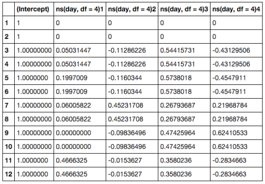
In order to pass the spline based model to Sleuth, we need to make a design matrix. This can be done by using the splines library and pass a formula using the splines by the ns() functions to model.matrix.

library(splines)
day <- s2c$day
full_design <- model.matrix(formula(~ ns(day, df = 4)))
full_design

The df parameter essentially governs how smoothed the expression patterns will be over the time points. I picked 4 because it’s the default in Ballgown. In Monocle the default is 3, but it seems this smooths the expression too much. Lower values for the df parameters will capture less “dynamics”, but will have more statistical power.

As described in the Sleuth vignette, it is quite handy to have the external gene name which is associated to every transcript, to quickly see roughly what gene we are looking at when we see a differentially expressed transcript.

library("biomaRt")
mart <- biomaRt::useMart(biomart = "ENSEMBL_MART_ENSEMBL",
dataset = "mmusculus_gene_ensembl",
host = "www.ensembl.org")
t2g <- biomaRt::getBM(attributes = c("ensembl_transcript_id",
"ensembl_gene_id",
"external_gene_name"),
  mart = mart)
t2g <- dplyr::rename(t2g,
target_id = ensembl_transcript_id,
ens_gene = ensembl_gene_id,
ext_gene = external_gene_name)

Now we are read to start performing the Sleuth analysis

so <- sleuth_prep(s2c, full_model = full_design, target_mapping = t2g)
so <- sleuth_fit(so)
so <- sleuth_fit(so, formula = ~ 1, fit_name = "reduced")
so <- sleuth_lrt(so, "reduced", "full")

Sleuth has an interactive Shiny application associated with it to browse the results of the analysis. It’s not mandatory to use it though, and many of the handy features in it mostly makes sense for the treatment-vs-control style of experiments.

plot_qq(so, test = 'reduced:full', test_type = 'lrt', sig_level = 0.05)

We can extract the results of the likelihood ratio test as a dataframe to look at closer

lrt_results <- sleuth_results(so, 'reduced:full', test_type = 'lrt')
table(lrt_results[,"qval"] < 0.05)

FALSE  TRUE 
49523  3083

This tells us that we find 3083 transcripts which have an expression pattern ove the time course which is significantly better explained by a natural spline over the time than by just random noise. Let’s have a look at the very top transcripts.

lrt_results %>% head(n = 20) %>% dplyr::select(target_id, qval, ens_gene, ext_gene)

I don’t know enough about brain development to say if these genes make any sense in the context. We can also plot a clustered heatmap of these top genes.

plot_transcript_heatmap(so, head(lrt_results, n = 20)$target_id, 'est_counts')

Unfortunately there doesn’t seem to be a way to rename the axis labels to some other information, or to enforce ordering the samples by time point. Let’s also plot the expression of a differntailly expressed transcript to see what it looks like.

tmp <- so$obs_raw %>% dplyr::filter(target_id == 'ENSMUST00000145067')
tmp <- dplyr::full_join(so$sample_to_covariates, tmp, by = 'sample')
tmp

tmp <- transform(tmp, day = as.numeric(day))
ggplot(tmp, aes(x=day, y=est_counts)) 
  + geom_point(shape=1) 
  + geom_smooth(method = loess)