Disappointing variational inference for GLMM's

Generalized linear mixed models (GLMMs) are fantastic tools for analyzing data with complex groupings in measurements. With a GLMM, one can write a model so that population level effects can be investigated and compared, while accounting for variation between groups within the population. As the number of population effects one wants to compare increases, and the size of the input data increases, the models take more time to fit.

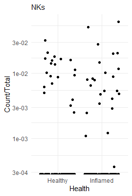
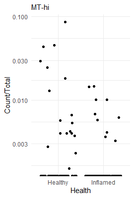
In Boland et al 2020 the authors compared mRNA expression in cells from blood and rectum from healthy people and patients with ulcerative colitis (UC). They found that T cells (specifically regulatory T cells) from rectum of UC patients had enriched expression of ZEB2. Estimating the expression levels of ZEB2 in the different conditions in this data is a good example of how GLMM's can be used.

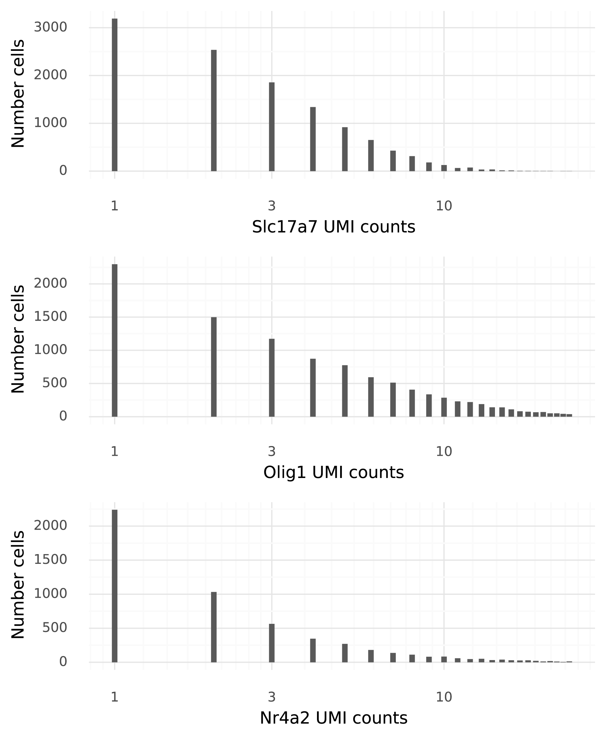
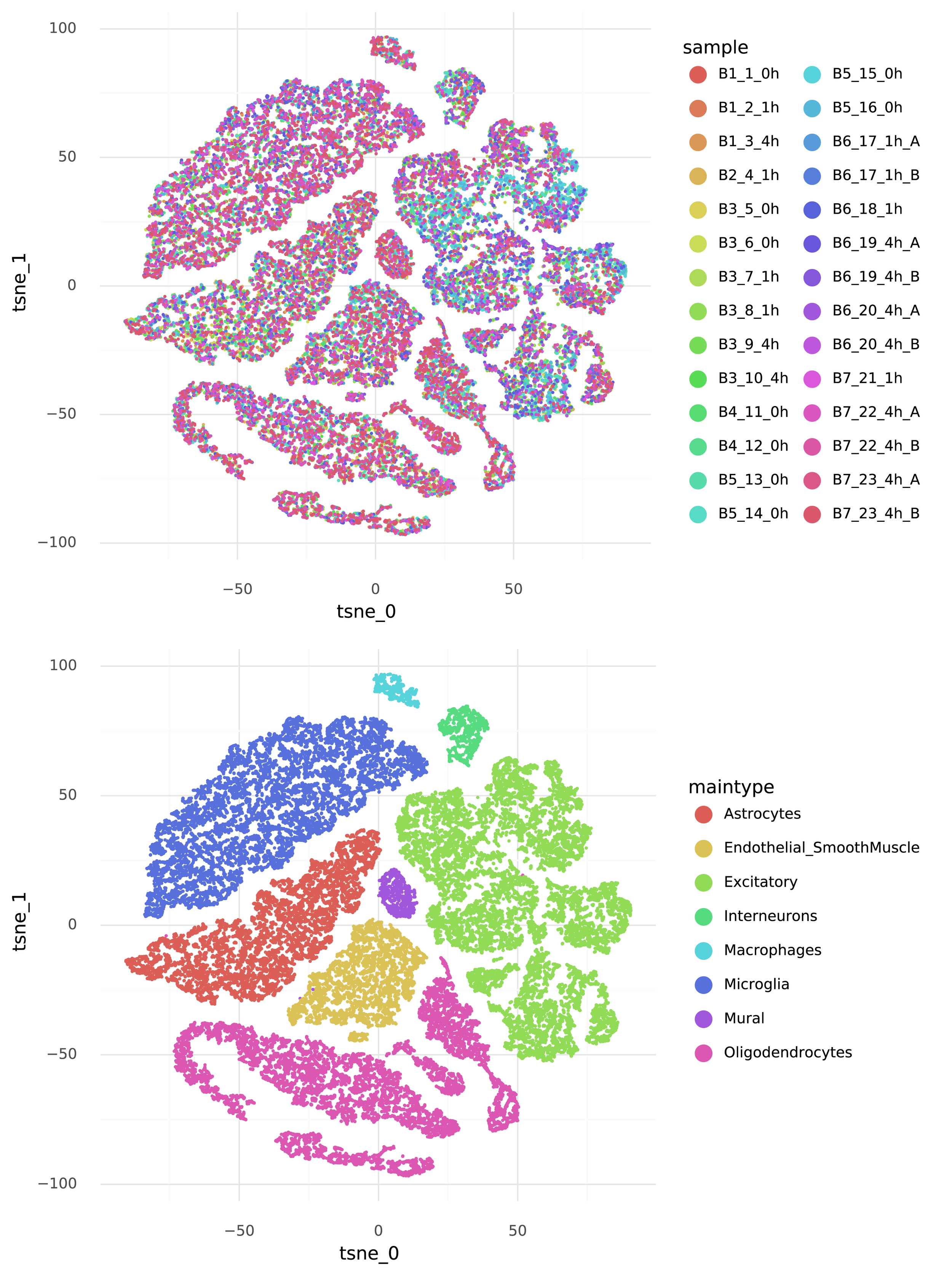
All the 68,627 cells in the Boland et al 2020 data can be divided into 20 cell groups of interest from the triplets (5 cell types, 2 tissues, 2 disease states). The cells were collected from 7 UC patients and 9 healthy people. Naturally, disease state is confounded with patient identity: with a regular generalized linear model it is not possible to account for patient-to-patient variation while estimating the disease state specific expression. However, with a GLMM, the patient-specific effect on the expression level can be considered a random effect while the disease state-specific expression level is a population effect. The GLMM for ZEB2 counts \( Y \) can be written as:

$$ \begin{align} \mu_\text{patient} &\sim \text{N}(0, \sigma_\text{patients}), \\ \lambda &= \exp(\mu_\text{cell group} + \mu_\text{patient} ) \cdot s, \\ Y &\sim \text{Poisson}(\lambda), \end{align} $$

where ( s ) is the UMI count depth per cell. This model can be fitted with the lme4 R package using the formula ZEB2 ~ 0 + cell_group + offset(log(total_count)) + (1 | patient_assignment). In the context of single cell RNA-seq data, this problem is relatively simple. There are only 20 fixed (population) effects, and 18 random effects, with ~70,000 observations. But it still takes over 15 minutes to fit this model of ZEB2 expression using lme4.

A popular method to scale model fitting is variational inference. Variational inference is a Bayesian method, so priors need to be specified:

$$ \begin{align} \sigma_\text{patients} &\sim \text{HalfNormal}(0, 1), \\ \mu_\text{cell group} &\sim \text{N}(0, 1) \end{align} $$

Tensorflow-probability (TFP) has a tutorial on how to fit GLMMs with variational inference on their website. The example code provided can be modified to implement the model defined above for the Boland et al 2020 data.

Unlike the parameter fitting algorithm in lme4, variational inference in TFP involves stochastic steps. To compare the results from lme4 with the results from the TFP model it is necessary to fit the TFP model several times to see how much the results vary between runs. Here, the TFP GLMM implementation was fitted on the Boland et al 2020 data 10 times.

The main goal is to obtain accurate estimates with uncertainty for the population level effects (the cell group means). Secondarily, it is good if the fits for the means of the random effects are accurately estimated.

Below are the estimated cell group means from lme4, and the 10 runs of TFP.

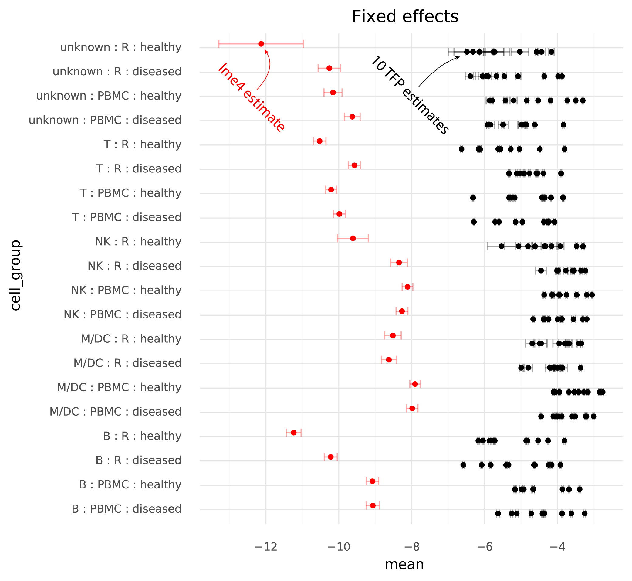
One immediately clear issue here is that there is a bias in the TFP estimates compared to the lme4 estimates. Looking at the random effects reveals the reason for this.

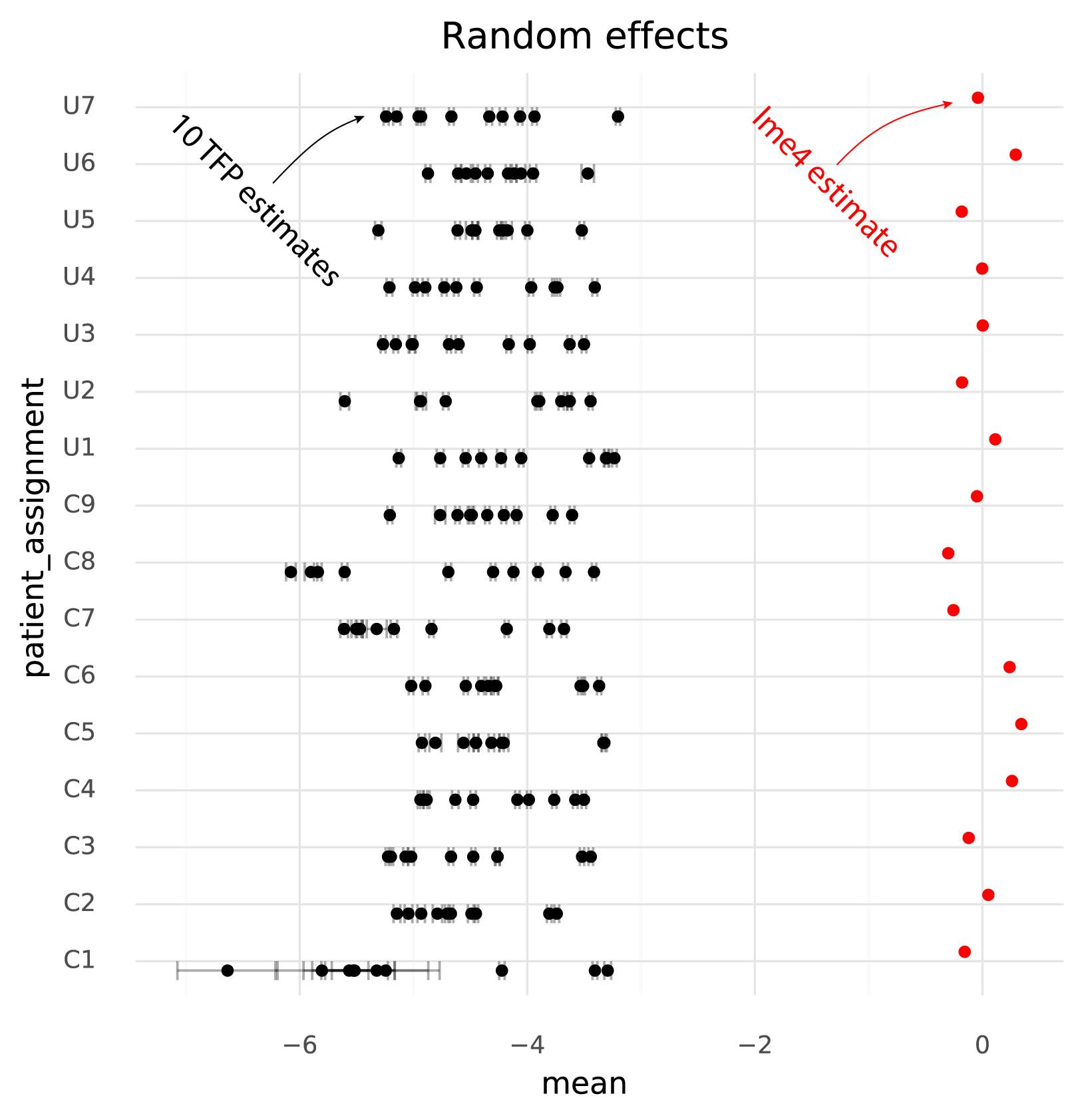
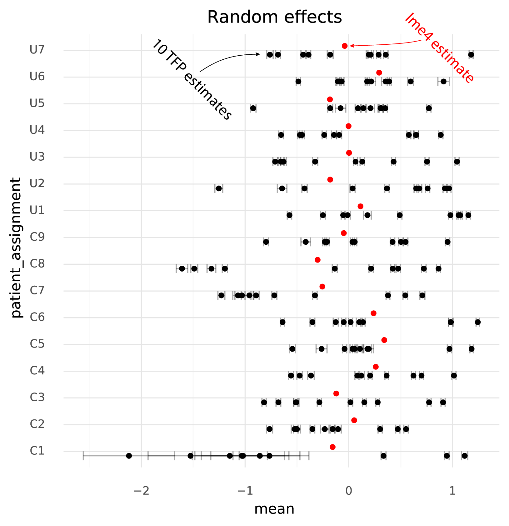
Even though the model specified \( \mu_\text{patient} \sim \text{N}(0, \sigma_\text{patients}) \) the TFP fits find a non-zero mean for the random effects. This might be an effect of the \( \text{N}(0, 1) \) prior on the fixed effects, causing the estimates both for the fixed and random effects to be shifted to satisfy both priors.

The units of the estimated fixed effects from TFP can be made comparable with the units from lme4 by shifting by the mean of the estimated random effects from TFP, since in the lme4 results the random effects have mean 0.

The following plot shows TFP fixed effect estimates on the transformed scale where the means of the random effects are 0:

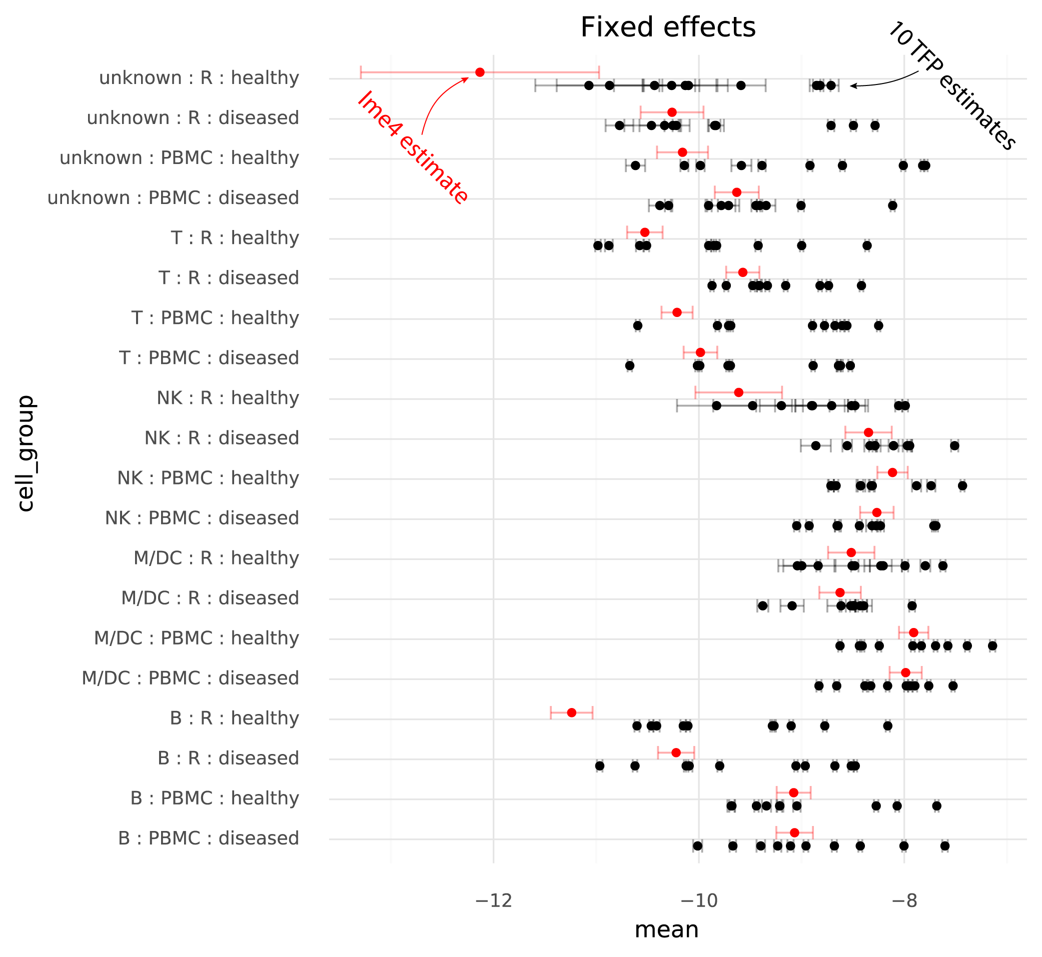
On this common scale (where the unit is “log probability of observing a ZEB2 molecule when sampling a molecule from the given cell group population”), there are two particularly clear issues. First, the whiskers on the plots show the +/- 2 * standard deviation of the estimates. The standard deviation of the lme4 estimates are obtained from the curvature of the likelihood function. The standard deviations from TFP are parameters which are fitted by the variational inference method. TFP standard deviations are much smaller than the standard deviations from lme4, reflecting a known property of variational inference.

Secondly, and more problematically, there is a huge amount of variation between runs of variational inference with TFP. This variation is much larger than the uncertainty in the lme4 estimate, and often changes the relative difference between two cell groups. That is, if one wants to calculate a contrast between two populations to perform a differential expression analysis, different runs of variational inference will result in negative or positive fold changes randomly.

This is disappointing, because these limitations are not discussed in the TFP tutorial on GLMM's. Instead, the TFP tutorial gives the impression that it 'just works', even without tuning the model.

Jupyter notebooks, R code, as well as a CSV file with ZEB2 expression data, are available at GitHub.

Cell type abundance analysis in scRNA-seq

By clustering, thresholds based on marker genes, or label transfer, cells in single-cell RNA-seq data can be assigned cell type labels. One use of scRNA-seq data is to compare abundance of cell types between experimental conditions or tissues. If a cell type is enriched in a disease condition it is an interesting avenue to explore what causes this increase in abundance.

Generalized linear models give a very simple yet powerful framework to study differences in cell type abundance. Each cell type can be considered to be sampled from a population of cells in an experimental sample.

Using a binomial linear model one can analyse counts of repeated observations of binary choices.

$$ N_{\text{cell type in sample}} \sim \text{B}(p, N_{\text{total cells in sample}}) $$ $$ \text{logit}(p) = \beta X $$

There are a large number of packages that can analyze this kind of model. They all differ slightly in how to provide values. The glm package in R takes these counts as paired observations of the form \( (N_{\text{cell type in sample}}, N_{\text{other cells in sample}}) = (N_{\text{cell type in sample}}, N_{\text{total cells in sample}} - N_{\text{cell type in sample}}) \).

To illustrate how a binomial GLM can be used to analyze cell type count data we use data from Smillie et al. Here the authors have 51 cell types (‘Cluster’) from a total of 365,492 cells from a number of individuals in healthy, non-inflamed, and inflamed states of ulcerative colitis. How can we analyze which cell types are enriched in inflamed samples?

By taking the metadata of the cells published with the paper, we can group the samples and count how many of each cell type are in each sample. For the input to the binomial GLM, we also calculate the total number of cells in each sample, and create an ‘Other’ column which have the number of cells in the sample not from the cell type of interest.

   Health  batch Location Subject Cluster               Count Total Other
   <chr>   <chr> <chr>    <chr>   <chr>                 <dbl> <dbl> <dbl>
 1 Healthy 0     Epi      N8      Best4+ Enterocytes       21   932   911
 2 Healthy 0     Epi      N8      CD4+ Activated Fos-hi     0   932   932
 3 Healthy 0     Epi      N8      CD4+ Activated Fos-lo     0   932   932
 4 Healthy 0     Epi      N8      CD4+ Memory               0   932   932
 5 Healthy 0     Epi      N8      CD4+ PD1+                 0   932   932
 6 Healthy 0     Epi      N8      CD8+ IELs                 0   932   932
 7 Healthy 0     Epi      N8      CD8+ IL17+                0   932   932
 8 Healthy 0     Epi      N8      CD8+ LP                   0   932   932
 9 Healthy 0     Epi      N8      CD69+ Mast                0   932   932
10 Healthy 0     Epi      N8      CD69- Mast                0   932   932

As a warmup, let us use a GLM to estimate the proportions of the cell types across all the samples, treating the samples as replicates. In this case a simple model can be made where Count vs Other only depends on the cell type identity

model0 <- glm(
  formula = cbind(Count, Other) ~ Cluster,
  family = binomial(link = 'logit'),
  data = df_a
)

An extremely useful tool when working with GLMs is the emmeans package. This package can transform a parameterization of a linear model to return any mean or contrast that is of interest. From the data and the simple linear model, we can obtain per-cell-type probability values with emmeans

emm0 <- emmeans(model0, specs = ~ Cluster)
emm0 %>%
  summary(infer = TRUE, type = 'response') %>%
  arrange(prob) -> cell_type_probs

cell_type_probs %>% head

            Cluster         prob           SE  df    asymp.LCL    asymp.UCL    z.ratio p.value
1        CD69- Mast 0.0003912534 3.271185e-05 Inf 0.0003321153 0.0004609172  -93.80333       0
2 Cycling Monocytes 0.0009576133 5.116207e-05 Inf 0.0008624047 0.0010633216 -129.96235       0
3            RSPO3+ 0.0009904458 5.203089e-05 Inf 0.0008935369 0.0010978534 -131.52763       0
4         CD4+ PD1+ 0.0011409278 5.583960e-05 Inf 0.0010365643 0.0012557858 -138.26581       0
5               DC1 0.0011710243 5.657044e-05 Inf 0.0010652300 0.0012873120 -139.53652       0
6           M cells 0.0012065928 5.742212e-05 Inf 0.0010991312 0.0013245468 -141.00855       0

The results can be compared with a much simpler strategy to get the cell type proportions: counting the cells per cell type in the data and dividing by the total number of cells.

df_a %>% pull(Count) %>% sum -> N
df_a %>% 
  group_by(Cluster) %>% 
  summarise(fraction = sum(Count) / N) %>% 
  arrange(fraction) %>% 
  as.data.frame -> cell_type_fractions

cell_type_fractions %>% left_join(cell_type_probs) -> cell_type_probs

So why bother with the GLM? Because with the GLM we can make predictors for cell type proportions that depend on predictors of interest (inflamed vs healthy), as well as accounting for batch effects and making use of replicates.

The ‘Health’ variable in the data contains ‘Healthy’, ‘Non-inflamed’ and ‘Inflamed’. For the sake of simplicity we will just consider ‘Healthy’ and ‘Inflamed’ here, so filter out ‘Non-inflamed’ samples.

We want to compare ‘Healthy’ and ‘Inflamed’ while accounting for variation due to ‘Location’ and ‘batch’. We do this by making a more complicated linear model

df_a %>% filter(Health %in% c('Healthy', 'Inflamed')) -> df
formula = cbind(Count, Other) ~ Cluster * Health + Cluster * Location + Cluster * batch
model1 <- glm(formula = formula, family = 'binomial', data = df)

Here the abundance of a given cell type depends on whether ‘Health’ is ‘Inflamed’ or ‘Healthy’. In addition, the abundance of the same cell type depends on ‘location’ and ‘batch’. After fitting the model we can compare odds ratios of ‘Inflamed’ vs ‘Healthy’ for each ‘Cluster’ using emmeans.

emm1 <- emmeans(model1, specs = revpairwise ~ Health | Cluster)
emm1$contrasts %>%
  summary(infer = TRUE, type = 'response') %>%
  rbind() %>%
  as.data.frame() -> c_results

             contrast                  Cluster odds.ratio          SE  df  asymp.LCL  asymp.UCL      z.ratio       p.value
1  Inflamed / Healthy Inflammatory Fibroblasts 62.4847804 14.10944910 Inf 40.1391051 97.2704243  18.31182457  6.660029e-75
2  Inflamed / Healthy                  M cells 16.5045991  3.48168172 Inf 10.9154622 24.9555893  13.29039892  2.631714e-40
3  Inflamed / Healthy   Inflammatory Monocytes  4.1921875  0.40353981 Inf  3.4713953  5.0626433  14.88908404  3.880492e-50
4  Inflamed / Healthy                Pericytes  4.1163273  0.50315305 Inf  3.2393999  5.2306448  11.57588915  5.460220e-31
5  Inflamed / Healthy   Post-capillary Venules  3.1448881  0.19793669 Inf  2.7799134  3.5577803  18.20453090  4.751058e-74
6  Inflamed / Healthy                Cycling B  2.5302852  0.15369320 Inf  2.2462922  2.8501826  15.28333532  9.875431e-53
7  Inflamed / Healthy                       GC  2.3807061  0.21261039 Inf  1.9984290  2.8361086   9.71268497  2.662299e-22
8  Inflamed / Healthy              Endothelial  2.1209671  0.12396363 Inf  1.8914025  2.3783945  12.86422519  7.155584e-38
9  Inflamed / Healthy                CD4+ PD1+  1.9756741  0.25707939 Inf  1.5309286  2.5496212   5.23284107  1.669243e-07
10 Inflamed / Healthy               Follicular  1.9259575  0.03832100 Inf  1.8522954  2.0025490  32.94061154 5.765493e-238
11 Inflamed / Healthy           Myofibroblasts  1.8911035  0.12724192 Inf  1.6574584  2.1576845   9.46964966  2.807838e-21
12 Inflamed / Healthy          Enteroendocrine  1.7511544  0.23462541 Inf  1.3467211  2.2770429   4.18168012  2.893629e-05
13 Inflamed / Healthy                    Tregs  1.6836653  0.06086953 Inf  1.5684919  1.8072958  14.41023630  4.461813e-47
14 Inflamed / Healthy                     Tuft  1.6445042  0.15265295 Inf  1.3709489  1.9726441   5.35882535  8.376478e-08
15 Inflamed / Healthy              Enterocytes  1.6271677  0.06957659 Inf  1.4963580  1.7694126  11.38560877  4.932258e-30
16 Inflamed / Healthy               CD69+ Mast  1.5857281  0.06127444 Inf  1.4700675  1.7104885  11.93140033  8.119601e-33
17 Inflamed / Healthy              CD4+ Memory  1.4140279  0.02517604 Inf  1.3655348  1.4642431  19.45814530  2.486205e-84
18 Inflamed / Healthy                   Goblet  1.3441453  0.08543563 Inf  1.1867049  1.5224733   4.65311890  3.269516e-06
19 Inflamed / Healthy               CD8+ IL17+  1.2856555  0.15437166 Inf  1.0160588  1.6267858   2.09264426  3.638092e-02
20 Inflamed / Healthy          Immature Goblet  1.2676903  0.04573710 Inf  1.1811433  1.3605789   6.57435120  4.886577e-11
21 Inflamed / Healthy       Best4+ Enterocytes  1.1589660  0.06670085 Inf  1.0353384  1.2973557   2.56338886  1.036559e-02
22 Inflamed / Healthy                     Stem  1.1518704  0.07809549 Inf  1.0085400  1.3155704   2.08538999  3.703391e-02
23 Inflamed / Healthy              Macrophages  1.1339316  0.02410242 Inf  1.0876623  1.1821693   5.91330273  3.353151e-09
24 Inflamed / Healthy                     TA 1  1.0774633  0.02269981 Inf  1.0338785  1.1228854   3.54139389  3.980189e-04
25 Inflamed / Healthy               Cycling TA  1.0770687  0.02800200 Inf  1.0235606  1.1333739   2.85568871  4.294359e-03
26 Inflamed / Healthy                Cycling T  1.0412753  0.10986760 Inf  0.8467459  1.2804953   0.38333047  7.014748e-01
27 Inflamed / Healthy          WNT2B+ Fos-lo 2  1.0233590  0.05237077 Inf  0.9256941  1.1313281   0.45120147  6.518444e-01
28 Inflamed / Healthy                      NKs  0.9952119  0.05914589 Inf  0.8857849  1.1181571  -0.08076013  9.356327e-01
29 Inflamed / Healthy                     TA 2  0.9930944  0.02931542 Inf  0.9372677  1.0522462  -0.23474820  8.144042e-01
30 Inflamed / Healthy             Secretory TA  0.9134756  0.04545739 Inf  0.8285878  1.0070602  -1.81858714  6.897444e-02
31 Inflamed / Healthy                  CD8+ LP  0.8908214  0.01948936 Inf  0.8534303  0.9298506  -5.28437421  1.261352e-07
32 Inflamed / Healthy                   Plasma  0.8881827  0.01002867 Inf  0.8687427  0.9080576 -10.50176601  8.477899e-26
33 Inflamed / Healthy   Immature Enterocytes 2  0.8734444  0.03039523 Inf  0.8158571  0.9350966  -3.88832100  1.009401e-04
34 Inflamed / Healthy                     ILCs  0.6891946  0.07523673 Inf  0.5564414  0.8536194  -3.40977118  6.501740e-04
35 Inflamed / Healthy                      DC1  0.6608477  0.07781771 Inf  0.5246488  0.8324038  -3.51776226  4.352021e-04
36 Inflamed / Healthy   Immature Enterocytes 1  0.6592190  0.02539055 Inf  0.6112864  0.7109101 -10.81883637  2.803136e-27
37 Inflamed / Healthy            WNT2B+ Fos-hi  0.6524180  0.02751867 Inf  0.6006516  0.7086457 -10.12505367  4.277440e-24
38 Inflamed / Healthy                      DC2  0.5976786  0.03078289 Inf  0.5402905  0.6611622  -9.99342232  1.628598e-23
39 Inflamed / Healthy                 WNT5B+ 1  0.5906783  0.03069201 Inf  0.5334849  0.6540034 -10.13235991  3.969516e-24
40 Inflamed / Healthy                 WNT5B+ 2  0.5801389  0.02750838 Inf  0.5286530  0.6366391 -11.48299320  1.606219e-30
41 Inflamed / Healthy          WNT2B+ Fos-lo 1  0.5559970  0.02165505 Inf  0.5151334  0.6001021 -15.07112820  2.507935e-51
42 Inflamed / Healthy   Enterocyte Progenitors  0.4850947  0.01928310 Inf  0.4487353  0.5244001 -18.19846809  5.307127e-74
43 Inflamed / Healthy    CD4+ Activated Fos-hi  0.4497154  0.01155000 Inf  0.4276382  0.4729325 -31.11565882 1.479043e-212
44 Inflamed / Healthy    CD4+ Activated Fos-lo  0.4256359  0.01102951 Inf  0.4045582  0.4478117 -32.96301722 2.753587e-238
45 Inflamed / Healthy            Microvascular  0.3241644  0.03439802 Inf  0.2632946  0.3991065 -10.61609664  2.508316e-26
46 Inflamed / Healthy                   RSPO3+  0.3030192  0.04640930 Inf  0.2244415  0.4091071  -7.79569031  6.405731e-15
47 Inflamed / Healthy                     Glia  0.2698563  0.02237938 Inf  0.2293727  0.3174851 -15.79469705  3.384151e-56
48 Inflamed / Healthy               CD69- Mast  0.2300449  0.05171148 Inf  0.1480717  0.3573988  -6.53716643  6.269527e-11
49 Inflamed / Healthy        Cycling Monocytes  0.2278063  0.03064635 Inf  0.1750069  0.2965352 -10.99591380  3.998428e-28
50 Inflamed / Healthy                    MT-hi  0.2235797  0.02702011 Inf  0.1764261  0.2833362 -12.39519687  2.774635e-35
51 Inflamed / Healthy                CD8+ IELs  0.2130551  0.01009845 Inf  0.1941540  0.2337962 -32.62151756 2.031799e-233

We see that the most enriched cell types are ‘Inflammatory Fibroblasts’, ‘M cells’, and ‘Inflammatory Monocytes’. The results from emmeans are in the unit of odds ratios. ‘Inflammatory Fibroblasts’ have an odds ratio of 62.5, which means the odds of seeing an ‘Inflammatory Fibroblast’ in an ‘Inflamed’ sample is 62.5 times higher than seeing an ‘Inflammatory Fibroblast’ in a healthy sample.These results can be visualized as a volcano plot to compare statistical significance and odds ratio for each cell type.

We can also extract the mean abundance for each ‘Cluster’ from the model using emmeans with a different ‘specs’ parameter. After putting this together with the previous results we can make an MA-plot to relate odds ratio with the average abundance of each cell type.

emm2 <- emmeans(model1, specs = ~ Cluster)
emm2 %>%
  summary(type = 'response') %>%
  select(Cluster, prob) -> mean_probs

c_results %>% left_join(mean_probs) -> m_results

To see how enriched looks in the raw data, we can plot a couple of cell types as a fraction of all cells in a sample. This way we can illustrate how a highly enriched cell type looks, compared to a non-enriched cell type, compared to a highly depleted cell type.

Generalized linear models are great tools to analyse various observed counts and known conditions. The largest inconvenience with GLMs is keeping track of parameter names, and transforming parameters to create contrasts to answer questions. The emmeans package really supercharges analysis using GLMS by tracking variable names and transformations for you.

An R file and data for this analysis are available at Github.

A trip through the layers of scVI

The scVI package provides a conditional variational autoencoder for the integration and analysis of scRNA-seq data. This is a generative model that uses a latent representation of cells which can produce gene UMI counts which have similar statistical properties as the observed data. To effectively use scVI it is best to think of it in terms of the generative model rather than the “auto encoder” aspect of it. That the latent representation is inferred using amortized inference rather than any other inference algorithm is more of an implementation detail.

This post goes through step by step how scVI takes the cell representation and is able to generate scRNA-seq UMI counts.

In summary, the steps are:

\[ W = f(Z, c) \] \[ X = g(W), \] \[ \omega = softmax(X), \] \[ \Lambda = \omega * \ell, \] \[ Y \sim NB(\Lambda, \theta), \]

A very good example dataset is one by Hrvatin et al. This data consists of UMI counts for 25,187 genes from 48,266 cells, sampled from the visual cortex of 28 mice (in three experimental conditions).

To illustrate the generative process in scVI, each step will use three genes (where applicable) to illustrate how each step goes towards generating counts. These are: Slc17a7, a marker for excitatory neurons; Olig1, a marker for oligodendrocytes; and Nr4a2, a gene which activates expression in some cell types when the mice are receiving light stimulation. It is clear that these genes have heterogeneity beyond observational noise, which makes them good candidates for illustration.

Below are three histograms of the observed UMI counts of these genes. The x-axis shows UMI counts between 1 and 25 for the gene, and the y-axis shows how many cells in the raw data that number of UMI counts is observed in.

After the data generative process has completed, the goal is to obtain data with very similar histograms to these.

\( Z \in \mathbb{R}^{10} \)

The journey towards generating counts starts with the representation \( Z \). Each cell is represented by a 10-dimensional vector \( z_i \) which describes the structured heterogeneity in the data. The goal is that cells that are close together in this representation have similar transcriptomes. A nice thing with scVI is that it estimates a posterior distribution for each \( z_i \), but in this post the focus is on the mean of \( z_i \). It is not feasible to visualize the 10-dimensional representation of the data, but we can create a tSNE visualization of the \( Z \), and color it by information that was provided in the published dataset from Hrvatin et al.

Note how the cells group by cell type, but not by experimental sample.

\( W = f(Z, c) \in \mathbb{R}^{128} \)

scVI is a conditional autoencoder. This is what enables it to find a representation with the variation between batches accounted for. When generating data the first step is to introduce the batch-to-batch variation. This is done by taking a representation \( z_i \) and the batch \( c_i \) of the \( i \)’th cell, passing these through a neural network \( f() \), and producing an intermediate representation \( w_i \). As above, cells with similar 128-dimensional \( w_i \) representations will produce similar transcriptome observations. Again, we cannot feasibly visualize the 128-dimensional representation of the data, but we can produce a tSNE visualization which allows us to see which cells are close together.

Note that compared to the previous tSNE, here cells from the same biological replicate are lumped together. But this happens within variation due to cell type.

\( X = g(W) \in \mathbb{R}^{25,187} \)

At last, it is time to start to tie gene expression to the cells. To move from the 128-dimensional representation of the cells, a neural network \( g() \) is used to produce one real value per gene in that cell. For this particular dataset each \( x_i \) is 25,187-dimensional. Below figure shows the distribution of these \( x_i \) values for the three example genes across the 48,266 cells in the dataset.

Now variation in gene expression levels can be investigated. This is particularly clear in the bimodal nature of Slc17a7 expression, owing to the mixture of excitatory neurons and other cells. However, these numbers (on the x-axis) that are produced by \( g() \) have no direct ties to the observed data. It is not clear what a value of 3.0 means, for example. This step is here simply because naive neural networks can only map values to unrestricted real numbers. The next step remedies this.

\( \omega = softmax(X) \in \Delta^{25,187} \)

The original data is in UMI counts, and counts are modeled through frequencies and rates. To obtain a frequency from the \( X \)-values, scVI performs a softmax transformation so that the resulting \( \omega_i \) value for each cell sums to 1. The softmax transformation is defined as

\[ \omega_{i, g} = softmax(X_{i, g}) = \frac{\exp(X_{i, g})}{\sum_{k=1}^G \exp(X_{i, k})}. \]

Thus, each \( \omega_i \) lies on the simplex \( \Delta^{25,187} \). Now scVI has generated a value we can interpret.

The frequency \( \omega_{i, g} \) means that every time we would count a molecule in cell \( i \), there is a \( \omega_{i, g} \) chance that the molecule was produced by gene \( g \). These (latent) frequencies are the most useful values produced in scVI, and allows for differential expression analysis as well as representing gene expression on an easily interpretable scale. By convention, the frequencies can be multiplied by 10,000 to arrive at a unit of “expected counts per 10k molecules” for genes. This is similar to the idea behind TPM as a unit in bulk RNA-seq.

\( \Lambda = \omega \cdot \ell \in \mathbb{R}^{25,187} \)

To be able to generate samples similar to the observed data, another technical source of variation needs to be added. Different cells have a different total number of UMI’s. The frequencies above represent how likely we are to observe a molecule from a given gene when sampling a single molecule. The rate \( \Lambda_{i, g} \) represent the expected number of molecules produced by gene \( g \) in cell \( i \) when sampling \( \ell_i \) molecules. This value \( \ell \) is usually referred to as the “library size” or “total UMI counts”. (In scVI \( \ell_i \) is also a random variable, but this is a detail that is not important for the general concept described here.)

In analysis of scRNA-seq data, the total UMI count per cell is easily influenced by technical aspects of data. Unlike frequencies, the scales for a given gene are not directly comparable between cells.

\( Y \sim \text{NB}(\Lambda, \theta) \in \mathbb{N}_0^{25,187} \)

Finally, using the rates \( \Lambda_{i, g} \), the observational negative binomial model can be used to draw samples of UMI counts per cell \( i \) and gene \( g \). (The additional dispersion parameter \( \theta \) can be estimated with a number of different strategies in scVI, and can be considered a detail here).

This is the final step which makes the model generative. At this point, the goal is that a sample from the model with the inferred \( \Lambda \) from the entire dataset should be easily confused with the observed data. The below figure shows histograms for the three example genes of the observed data in grey, and from a sample from the scVI model in red.

An even better strategy to illustrate these properties is to draw multiple samples and see whether the observed data falls within certainty intervals of the sampled data. In the figure below each red line corresponds to a histogram value from a sample from the observational model.

The data and the samples have pretty similar distributions. Some aspects of the observed data are not seen in the samples from the observational model. In particular data sampled from the observational model produce more 1-counts for these three genes than what was observed in the data.

(It should be noted that here samples have only been taken at the last step, from the observational negative binomial model. To perform a posterior predictive check, \( Z \)-values should also be sampled from the approximate posterior of \( Z \).)

The aim of this post has been to show how in scVI the representation \( Z \), which can be used for many cell-similarity analyses is directly tied to gene expression. And the gene expression in turn is directly tied to the sparse UMI counts that are observed through single cell RNA-sequencing. These links are very difficult to make in other analysis methods or 'pipelines' of analysis.

A Juptyer notebook that illustrates how to generate all the quantities described here and all the figures is available on Github

Microphones for Zoom meetings

Since the lockdowns started in March, Zoom meetings have become an intgral part of of a typical workday. Like most people, I was just using my AirPods Pro, until I dropped one of them and something went wrong with the noise cancellation. They still work, but when I speak I hear myself echoed in the right earbud, which ended up being very annoying. I wanted to get a Blue Yeti USB microphone to replace them, but at this point they were all sold out. I figured a small simple solution would be to get a wireless lavalier mic. This is pretty much as unobtrusive as the AirPods Pro.

Unfortunately, I discovered the lavalier mic sounded terrible. Maybe because I got a pretty cheap one, but when using the "Test Mic" feature in Zoom with it I figured I wouldn't want to bother anyone with such bad audio. Instead I got a popular condensor microphone and an audio interface, the next best thing after a Blue Yeti USB microphone (which were still sold out).

When testing the condensor microphone in Zoom's "Test Mic" feature I was very disappointed, it sounded terrible. I tried recording the mic in Quicktime, and it sounded much better!

As a demonstration, here is a recording using a shotgun mic recorded directly from the source, and a captured recording of what the "Test Mic" feature sounds like in Zoom with the same microphone.

What I heard from the "Test Mic" feature sounded much worse than anyone had ever sounded in a Zoom meeting for me. I was wondering if my audio actually sounded that bad on the end of a receiver. To test this, I set up a Zoom meeting between my laptop and my desktop, and recorded microphone tests as they sounded on the receiving laptop transmitted from the desktop with the microphone plugged in. It turns out the "Test Mic" feature is nowhere near representative of the actual sound of the microphone over Zoom.

While I had this set up, I recorded several different options for microphones for the sake of a comparison. I also recorded local native microphone samples to learn in what ways Zoom distorts audio.

There are a number of options in Zoom to disable various audio filters, but I couldn't understand what they did, so I left them all on the defaults.

Here is the collection of all microphones I tested with this setup. Most interesting is probably the right hand column of audio clips that demonstrates what the different microphones sounds like over a Zoom meeting.

This taught me that the condensor microphone actually soundeed very good. But I had also gotten a shotgun microphone to replace my condensor microphone. While the condensor microphone has great sound, it is very large and needs to be very close to your mouth when using it. It was always covering my view of the screen and my keyboard, a shotgun microphone can be further away to not ubscure your view of the screen.

It turned out the wireless lavalier mic still sounded very bad, I'm not sure why. It is unfortunate, because it would definitaly be more convenient than a large wired microphone connected to an audio interface which takes up an annoying amount of desk space.

I was also surprised to learn the AirPods Pro sounds pretty bad over Zoom too. A common first tip for good Zoom meeting audio is to use any headset instead of the microphone built into your computer or webcam. But at least to my ears the built in microphones in my iMac, my webcam, and my laptop all sound better than than the AirPods Pro. This could be another symptom of them being slighly broken.

Taking all the recorded microphones, I ranked them by listening to them pairwise and deciding which one I thought sounded better. I also thought about which options were more convenient, using subjective considerations such as whether they are wired, comfortable, mobile, taking up space, etc. The figure below summarizes how I would rank the microphone options along both axes.

Zoom meetings are exhaustng, to the point where I have no interest what so ever to attend any of the upcoming remote versions of conferences. I feel very bad for students who have to endure remote school days and lectures. There are many reasons Zoom meetings are tiring, but I belieave a major reason is the poor audio quality from the people speaking.

This comparison helped me decide between my options. I wish wireless options were better so I could more easily take meetings away from my work desk to get some more variety into my workday.

Comparing Slide-seq and Slide-seqV2 counts

Slide-seq is a promising technology for the study of cellular tissue anatomy.It uses a clever strategy to randomly deposit barcoded RNA-capture beads on slides. To record the location of the beads the barcode is read off using in situ sequencing. Following this, a slice of tissue can be deposited on the slide, where the beads can capture RNA from the cells of the tissue. After this step the beads can be treated as from a Drop-seq experiment, and with high throughput sequencing one can arrive at a count matrix of beads x genes, with the paired information of spatial coordinates of the beads.

Slide-seq was published a year ago, and the dataset is still the largest published in terms of number of observations with 2,522,640 beads. The data ended up being difficult to analyze however, due to extremely low counts per bead. Even with very large numbers of observations it is difficult to learn structure in count data of counts are small.

Recently, an update called ‘Slide-seqV2’ was published. In the paper they describe testing Slide-seq and Slide-seq2 on serial sections of brain tissue and find a ten-fold improvement in average counts.

This is on newly generated data, and I was curious how the previous data compares. Relative improvement within an experiment tells you about how much better the protocol is, but what I wanted to know was how much easier this experiment would be to analyze. For this sequencing depth needs to be considered, which may not necessarily be matched between the old and the new data.

After downloading the data made public by the authors, I converted it, combined it with the old Slide-seq data, and made a plot comparing the number of counts per bead between the protocols. (I also live streamed this process, available here)

A simple analysis shows that for the Slide-seq data there are on average 40 UMI’s per bead, while the Slide-seqV2 data has 200 UMI’s per bead: a 5-fold increase. The Slide-seq2 data has a very wide spread of counts per bead.

Preferably you would have at least a few thousand UMI’s per observation when doing analysis. This is a step in the right direction, but it still might require the supervised style analysis presented in both the papers, which make use of additional scRNA-seq data as a guide.

The analysis is available on Github, and I have made available H5AD files containing the Slide-seq here and Slide-seq2 data here.

Converting images of line graphs to data

Recently Google released aggregated anonymized data on community mobility for 131 countries based on cell phone location data. The data spanned the time period between February 16 and March 29, and made clear how people have limited visits to places categorized as “Retail & recreation”.

The data was made available as line graphs in PDF reports per country, meaning you need to open each country you want to look at in a separate document. I wanted to see how population behaviour had changed globally by looking at many countries at the same time. But the data used to make the curves in the reports was not available for direct download.

In the PDF’s the curves are vector graphics, so in theory the underlying data is embedded within the PDF. Using Illustrator I could access the curve element, but I couldn’t see a way to extract the data that builds the curve. I tried finding tools explicitly made for extracting data from PDF’s and encountered a tool called “norma”, but I couldn’t get it to work.

The line graphs are pretty clear and have simple colors, so I thought it would be pretty simple to extract the values even if I had the bitmap images of the graphs.

I used Greenshot to take screenshots of the regions in the reports in the range -80% to 80%, which are the labeled extremes on the y-axis, while covering the entire x-axis.

After loading a screenshot in Python I could isolate the pixels belonging to the curve by using a threshold on the red channel.

These pixel values together with the knowledge of the axis scales can be used to recover the original data.

# Binarize the image
mask = 0.5 < img[:, :, 0]

# The `.argmin(0)` method will return the first index where
# we see a black pixel along the y-axis in the image.
# Images have negative y-axis, flip to get positive values.
pixel_value = -mask.argmin(0)

# We know the y-axis spans the interval [-80, 80]. To get the
# original values, scale values to the fraction of vertical pixels
# the observed values are at. Then scale these fractions to the
# [-80, 80] interval.
percent = 160 * (pixel_value + img.shape[0]) / img.shape[0] - 80

# The reported dates start on February 16 and end on March 29.
# Make a DateRangeIndex defined for a single day's resolution.
dates = pd.date_range(datetime.date(2020, 2, 16), datetime.date(2020, 3, 29))

daily_percent = (
    pd.DataFrame({
        # Use the `cut()` function to bin horizontal pixels into
        # intervals corresponding to the days.
        'bins': pd.cut(np.arange(percent.shape[0]), bins=dates.shape[0]),
        'percent': percent
    })
    # Group the percent values by the day bins.
    .groupby('bins')
    # Extract the median percent value for each bin.
    .median()
    .reset_index(drop=True)
)

# Finally, add the dates to the data
daily_percent['date'] = dates

Now we have the percentage values for each day in a DataFrame and can re-plot it to recreate the reported curve.

p.options.figure_size = (6, 4)
(
    p.ggplot(p.aes(x='date', y='percent'), daily_percent)
    + p.geom_line()
    + p.scale_y_continuous(limits=(-80, 80))
    + p.theme_minimal()
)

Having validated that it was possible to recover the data given the screenshots, I spent some time creating screenshots for 47 countries. With these I could simply loop over the images, create the DataFrames, and combine them at the end. With the combined data I was able to make the combined plot I wanted:

The notebook I used to do this, as well as a CSV of the resulting DataFrame, are available on Github.