Immune response enrichment analysis in Python

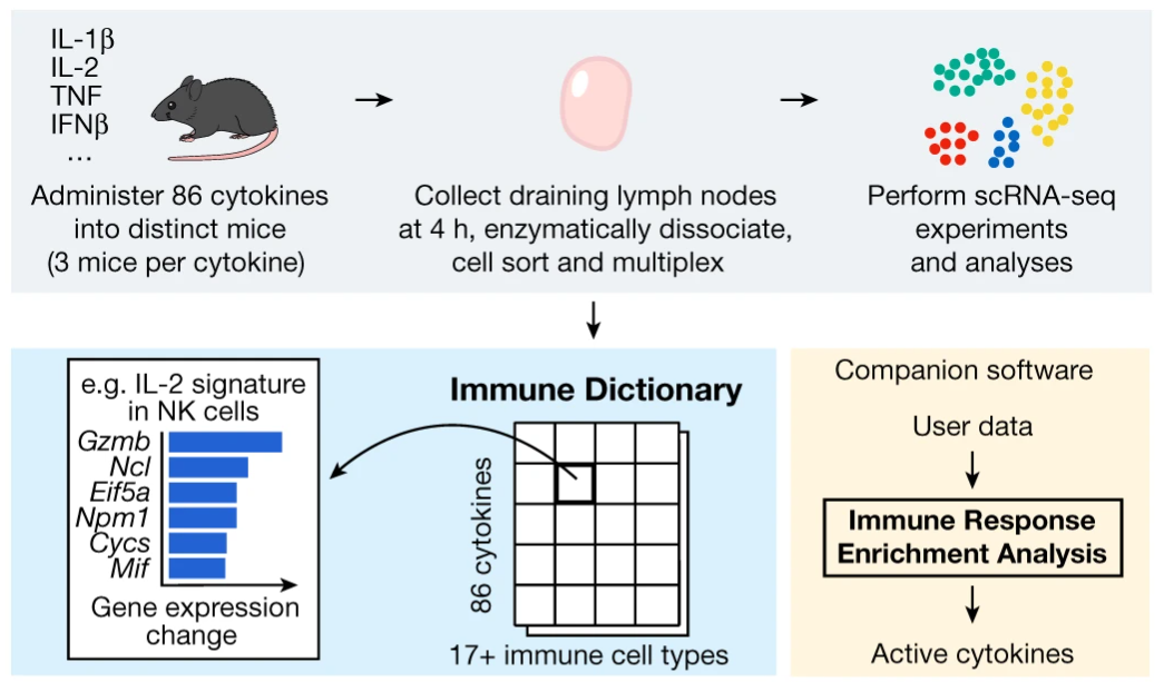
In a recent paper, Cui and colleagues define a ‘dictionary’ of immune responses to cytokine stimulation (Cui et al. 2023). The experiments performed to produce this dictionary is at an impressive scale, involving injecting 272 mice with 86 different cytokines and harvesting cells from the mice’s draining lymph nodes.

Cytokines are secreted proteins that interact with surface receptors of cells, signaling to the receiving cell to change its current state or perform a function. The immune system heavily relies on this form of signaling.

When a problem occurs, non-immune cells signal to immune cells to activate, to recruit them to the site of the problem, differentiate cells to properly respond to the problem. After the issue is resolved, other cytokines are secreted to decrease the activities of the responding cells. The immune system consists of many components, many different cell types which can handle immune issues in different ways. These components communicate with different sets of cytokines to customize the responses to the problem at hand (Altan-Bonnet and Mukherjee 2019; Saxton, Glassman, and Garcia 2022; Moschen, Tilg, and Raine 2019).

In any diseases or afflictions where the immune system is involved, it is extremely valuable to know which cytokines are involved. The immune dictionary by Cui and colleagues provides, for a large collection of cell type-cytokine pairs, the genes which are transcribed in response to the stimulation from that cytokine. If you know what cell type you are looking at, which genes that cell type has started transcribing, you can look up in the dictionary which cytokine stimulated the cell.

Adapted from https://www.nature.com/articles/s41586-023-06816-9/figures/1

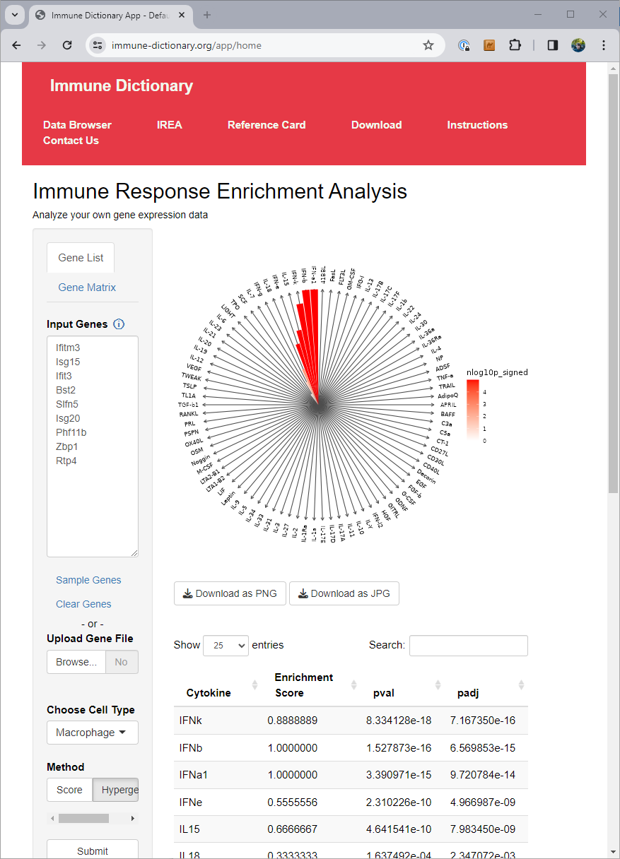
The authors of the immune dictionary created a website at https://www.immune-dictionary.org/ where anyone can upload a list of genes, and infer which cytokines are responsible for the expression of those genes, through what they call ‘immune response enrichment analysis’.


When working in cases with many different conditions or cell types, going to a website and pasting in gene lists for each of them can end up being tedious. At that point you want a solution you can just run as code in your local environment.

The final dictionary from Cui and colleagues, summarizing the results of their large experiment, is available as Supplementary Table 3 in the online version of the paper, having the filename 41586_2023_6816_MOESM5_ESM.xlsx. With these data the tests available on the immune-dictionary.org website can be implemented in Python.

For an example, I found a dataset of mouse colon tissue, with the three conditions of healthy, acute colitis, and chronic colitis, on Figshare. Unfortunately, I haven’t been able to identify what paper these data are from, but it has annotated cell type labels which is very useful for this analysis. By comparing macrophages from healthy mice with macrophages from mice with acute colitis, we can see which genes are activated in the acute colitis case, and compare that list of genes to the genes activated by the different cytokines in the immune dictionary.

After cleaning up the mouse colon data (changing gene identifiers) I ingested it into my Lamin database and fitted an SCVI model to use for differential expression tests.

After reading in the immune response dictionary gene lists from the Excel file, enrichment analysis is done by looking at the overlap between cytokine response genes and genes that are differentially expressed, using, for example, a hypergeometric test.

The Pertpy package’s Enrichment.hypergeometric function would probably be the easiest way to perform the analysis. The gene lists per cytokine stimulation are provided as a dictionary. This function requires your DE results to be stored in a specific format used by scanpy’s rank_genes_groups function.

Since I’m using an SCVI model for differential expression, it will be easier to just obtain a list of DE genes and make use of the code behind the Enrichment.hypergeometric function.

# Differential expression

idx_ = (
    vae.adata.obs
    .query('celltype_minor == "Macrophage"')
    .query('condition in ["Healthy", "AcuteColitis"]')
    .index
)
tmp_ = vae.adata[idx_].copy()

de_results = vae.differential_expression(
    tmp_,
    groupby = 'condition',
    group1 = 'AcuteColitis',
    group2 = 'Healthy'
)

fde_r = (
    de_results
    .query('proba_de > 0.95')
)


# Get immune dictionary gene lists

celltype_response = cytokine_responses.query('Celltype_Str == "Macrophage"').copy()
celltype_response['Gene'] = celltype_response['Gene'].map(lambda s: [s])
response_sets = celltype_response.groupby(['Cytokine'])['Gene'].sum().to_dict()


# Calculate hypergeometric gene set enrichment statistics

de_genes = set(fde_r.index)
universe = set(vae.adata.var.index)

results = pd.DataFrame(
    1,
    index = list(response_sets.keys()),
    columns=['intersection', 'response_gene_set', 'de_genes', 'universe', 'pvals']
)
results['de_genes'] = len(de_genes)
results['universe'] = len(universe)

for ind in results.index:
    response_gene_set = set(response_sets[ind])
    common = response_gene_set.intersection(de_genes)
    results.loc[ind, "intersection"] = len(common)
    results.loc[ind, "response_gene_set"] = len(response_gene_set)
    pval = stats.hypergeom.sf(len(common) - 1, len(universe), len(de_genes), len(response_gene_set))
    results.loc[ind, 'pvals'] = pval

results['Cytokine'] = results.index

After this we can investigate the results table, or, here, to save some space, visualize the ranking of likely upstream cytokines in a plot.

|        |   intersection |   response_gene_set |   de_genes |   universe |      pvals | Cytokine   |
|:-------|---------------:|--------------------:|-----------:|-----------:|-----------:|:-----------|
| IL-21  |              1 |                   1 |         96 |      18416 | 0.00521286 | IL-21      |
| RANKL  |              1 |                   1 |         96 |      18416 | 0.00521286 | RANKL      |
| IL-13  |              2 |                  34 |         96 |      18416 | 0.0135363  | IL-13      |
| IL-17F |              1 |                   3 |         96 |      18416 | 0.015558   | IL-17F     |
| OSM    |              1 |                   7 |         96 |      18416 | 0.0359301  | OSM        |
...

We see that, based on the immune dictionary, the macrophages in the colon of mice with acute colitis are likely to have been stimulated by the cytokines IL-21, RANKL, IL-17F, IL-13, and OSM.

The notebooks used for this post are available on GitHub, the data used for this post are available on LaminDB, and the trained SCVI model is available from Hugging Face using scvi-hub. Thanks to Eduardo Beltrame for helpful feedback on this post.

References

Altan-Bonnet, Grégoire, and Ratnadeep Mukherjee. 2019. “Cytokine-Mediated Communication: A Quantitative Appraisal of Immune Complexity.” Nature Reviews. Immunology 19 (4): 205–17. https://doi.org/10.1038/s41577-019-0131-x.

Cui, Ang, Teddy Huang, Shuqiang Li, Aileen Ma, Jorge L. Pérez, Chris Sander, Derin B. Keskin, Catherine J. Wu, Ernest Fraenkel, and Nir Hacohen. 2023. “Dictionary of Immune Responses to Cytokines at Single-Cell Resolution.” Nature, December. https://doi.org/10.1038/s41586-023-06816-9.

Moschen, Alexander R., Herbert Tilg, and Tim Raine. 2019. “IL-12, IL-23 and IL-17 in IBD: Immunobiology and Therapeutic Targeting.” Nature Reviews. Gastroenterology & Hepatology 16 (3): 185–96. https://doi.org/10.1038/s41575-018-0084-8.

Saxton, Robert A., Caleb R. Glassman, and K. Christopher Garcia. 2022. “Emerging Principles of Cytokine Pharmacology and Therapeutics.” Nature Reviews. Drug Discovery, September. https://doi.org/10.1038/s41573-022-00557-6.
Single-cell metadata as language

Single-cell RNA-seq data is molecule counts of transcripts from different genes within different cells. With this data alone, you can learn which genes tend to covary between cells, or you might learn of groups of cells where different sets of genes are used.

Metadata is data about this data. In the single-cell field this includes information such as which tissue were the cells were harvested from, what technology was used to perform the measurements, or was there some experimental stimulation of the cells.

When you are relating the data and the metadata, you get a connection between the gene expression patterns and external phenomena. You can relate the observations to the rest of the world, either in terms of what observations are related to technical factors, or how observations might change depending on stimuli.Only when you have both gene expression data and the sources of variation in the data can you begin to understand how gene expression is modified in the cells, or the expression in the cells lead to related downstream differences.

When working with single-cell data from multiple sources, you quickly encounter the issue of different people having different ideas on how to format the metadata for the cells. For example, below are the metadata fields and values for two cells from two different data sets.

{
    "Index": "CTGAAACAGAATAGGG-11",
    "Patient_assignment": "U3",
    "Tissue_assignment": "R",
    "Disease_assignment": "diseased",
    "Celltype": "B"
}

{
    "Index": "N52.LPA1b.CCCAGTTTCTGGTTCC-2",
    "Cluster": "Plasma",
    "Subject": "N52",
    "Health": "Non-inflamed",
    "Location": "LP",
    "Sample": "N52.LPA1b",
    "Batch": "2"
}

In any analysis of data from the two datasets, the metadata needs to be harmonized. You will need to assign a relation between what parts of data represent the same thing, or different things. Which fields relate to the same concept (e.g., ‘Celltype’ and ‘Cluster’)? Which values within a field represent the same category (e.g., plasma cells are a subset of B cells)?

Once metadata in different datasets are harmonized, and there are subsets of data that are aligned, the different datasets can be put in a model, treated as replicates, or used for comparisons. This metadata harmonization work is equally required no matter the analysis workflow, no matter if it is based on linear models, graph based methods, nonparametric statistics, or deep generative models. The concepts in the metadata need to be aligned to a common vocabulary.

When you are looking at the metadata examples from two cells above, you are probably already aligning the concepts in your head. Clusters and cell types, health status, there appears to be multiple patients and batches which can probably be treated as replicates, etc.

Why can you do this matching? It is because even though the metadata is not standardized, it is text communicating language, in a somewhat structured way. The people who wrote this metadata did actually write it in a way meant to communicate information. They just had slightly different ideas about phrasing. The metadata is language.

At this moment, there are endless language models that can take pieces of text and produce embedding vectors which preserve semantic relations between the texts, in contexts all the way between song lyrics and code in obscure programming languages. These embedding models are designed to preserve that intuition about relations between text which we are using when we can match up the concepts in the metadata examples above.

If we can convert the metadata for the cells to vector representations that preserve the information that the original author meant to communicate, then we can redefine an enormous amount of analysis tasks to circumvent the harmonization step.

A simple version of metadata embedding could be to take the metadata dictionary, convert it to a JSON string, and embed this with a language embedding model, e.g., text-embedding-3-small from OpenAI.

client = OpenAI()

row_ = pd.Series({
    "Index": "CTGAAACAGAATAGGG-11",
    "Patient_assignment": "U3",
    "Tissue_assignment": "R",
    "Disease_assignment": "diseased",
    "Celltype": "B"
})

js_ = row_.to_json()

response = client.embeddings.create(
        input = js_,
        model = 'text-embedding-3-small'
    )

embeddings = np.array([d.embedding for d in response.data])

To investigate this strategy, I went through my collection of scRNA-seq data and sampled 100 random cells from each dataset. I filtered out all cells that didn’t have textual metadata, and was left with 5,760 cells from 58 datasets. I took the textual metadata (that is, I filtered out numeric metadata) for these cells and created 1,536-dimensional embeddings of the JSON representations using the text-embedding-3-small model.

To get some intuition about the embeddings, they can be visualized with PyMDE.

Cell metadata from the same dataset largely group together and do not intermix. There are some cases where we can see the same dataset occupy different regions in the embeddings (for example, purple data in lower right corner).

Do the embeddings represent any interesting information within datasets? As an example, we can zoom in on the first dataset as an example (this is the data with the first dictionary of the first example up top).

These cells have metadata that cover three distinct regions in the embedding space.

Coloring the cells by some of the metadata information (PBMC vs R [rectum], diseased vs healthy), we can see that the metadata embedding is reflecting that these cells came from different tissues and different disease states.

So, what do these figures indicate? They are pointing to some interesting analysis strategies.

When integrating out variation between datasets, the common choice is a one-hot encoded vector of the length of the number of datasets. Since individual datasets appear to group together in distinct space, the embedding coordinates could be used as continuous covariates in integration models.

Within a dataset, cells with different recorded properties are separated. So also on the local scale, within-dataset, between-condition variation can be modeled with the embedding coordinates as covariates.

This concept can be used with many analysis strategies, but it would tie well with the conditional variational autoencoders in scvi-tools. Zooming in on the relevant part of the SCVI model, a model can be defined with $$ \rho_n = f(z_n, s^{\text{dataset}}_n, s^{\text{health}}_n), $$

where \( s^{\text{dataset}} \) and \( s^{\text{health}} \) end up being one-hot encodings of the dataset and health categories.

Instead, we can imagine creating the cVAE so that it is conditional on the metadata embedding vector (from some function \( g \)):

$$ \rho_n = f(z_n, g(\text{metadata})). $$

This way, we can tie the gene expression to the author-reported language in the cell metadata. We can analyze the data without spending as much time on metadata harmonization.

There are more potential benefits. We have been thinking about using the language embeddings as a way to represent the observed metadata. Another concept is that the observed language in the metadata can be related directly to language as queries about the data.

The example dataset above mentions two tissue sources for the cells: PBMC, and R. As an example, we can take just the English word “Blood”, and ask how similar the different cells metadata are to this word. Coloring the cells by their metadata distance to “Blood” we see that PBMC-cells are closer than R-cells. We are not informing the model that PBMC is a subset of blood, instead this information is encoded in the OpenAI language model and represented in the embeddings.

This suggests that if a model is trained with enough single cell data with matched embedded metadata we could get to a point where we can ask differential expression queries using natural language. You can imagine using different natural language queries to filter areas in \( Z \) cell transcriptome representation space and define contrasts between areas of metadata embedding space, leading us to highly complex conditional questions.

Here I have just tested a raw embedding of the JSON of the metadata. I couldn’t find any models that had been specifically trained to represent key-value dictionaries. It would be interesting if the language model had distinctions between keys and values encoded in it somehow, though I’m not sure in what way.

Another potential direction could be to fine-tune the language embedding model as the gene expression cVAE model is trained. By iterating between training the cell gene expression representation model and training the metadata embedding model, some gene expression information will inform which terms in the metadata are similar.

A notebook with the analysis presented here is available on GitHub. Thanks to Eduardo Beltrame for helpful feedback on this post.

Organizing scRNA-seq data with LaminDB

Occasionally, when I’m curious about something scRNA-seq related, I analyze some data. Often this leads to posts on this website.

I have made it a habit to try to find some recent, somewhat interesting, scRNA-seq data for these kinds of analysis. This is because I don’t want to end up mentally overfitting to a particular dataset, and I also consider it a way to keep up with how the scale and complexity of datasets are changing over time.

Over the years, I have ended up collecting a large number of scRNA-seq datasets. I did a global search for ‘*.h5ad’ on my Google Drive, and found over 300 files in various directories scattered throughout my drive.

Due to the increasing popularity and scale of scRNA-seq experiments, products for organizing large collections of data, such as LaminDB.

LaminDB is designed for tracking biological data in general. It offers plugins to manage ontologies related to scRNA-seq data as well as for AnnData format data.

The LaminDB database tracks metadata about the data, as well as the location of the data. It can track data locally on a computer, but it is probably most useful when storing your data on cloud storage.

After filtering duplicates and non-public H5ADs from my list, I ingested all my H5ADs into LaminDB, while also spending some time to hunt down the original publications for all the datasets and tag them with the DOI of the source publication for each dataset.

LaminDB is organized around ‘artifacts’ and ‘collections’. Each H5AD file is considered an ‘artifact’, which can be annotated with ‘features’ and ‘labels’.

Since each artifact (H5AD file) has an article DOI associated, I was able to use the single cell studies database to add some further annotation to the files: organism, tissue, and technique associated with the DOI.

Features and labels can be arbitrarily registered, and you can build your own ontologies to organize your data. For single-cell genomics data, Lamin provides a plugin, ‘bionty’, with pre-defined labels and features using relevant public ontologies, including organisms and tissues. The data from the single cell studies database was used to create these labels for the artifacts.

The LaminDB database can be explored on lamin.ai, and can be loaded by running lamin load vals/scrna in the terminal. In my case, the database is hosted on AWS. After running the load command, the database is directly accessible in Python through the ‘lamindb’ package, which is typically imported as ln.

For example, we can count how many files are tracked by the database.

> ln.Artifact.filter().all().count()
236

These are the 236 H5AD files I ingested to the database after deduplication. This deduplication happened automatically as I ingested files based on the hash of the file contents.

Files of interest can be identified by filtering based on metadata (which in this case is on the publication level).

> organisms = lb.Organism.lookup()
> tissues = lb.Tissue.lookup()
> techniques = lb.ExperimentalFactor.lookup()
> query = (
    ln.Artifact
    .filter(organism = organisms.mouse)
    .filter(tissues = tissues.brain)
    .filter(experimental_factors = techniques.chromium)
)

> print(query.df().head())
                     uid  storage_id   
id                                     
15  88k1xpSWBdJzEbYUf6MZ           1  \
16  UDH0CAo3JHo0uQUiAtUV           1   
21  kFvwhKtIBY0mhQTOqaOX           1   
22  PBAwUla9eERbI1KJQADZ           1   
23  HW9uS90M2PVyeX50o6ct           1   

                                                  key suffix accessor   
id                                                                      
15      cortex-align-2018/Zeisel 2018/l1_cortex2.h5ad  .h5ad  AnnData  \
16      cortex-align-2018/Zeisel 2018/l1_cortex3.h5ad  .h5ad  AnnData   
21  hca-benchmark-2019/Ding/2019-05-Ding-et-al-bio...  .h5ad  AnnData   
22  hca-benchmark-2019/Ding/PBMC/PBMC_read_counts....  .h5ad  AnnData   
23  hca-benchmark-2019/Ding/PBMC/PBMC_umi_counts.h5ad  .h5ad  AnnData   

   description version       size                    hash hash_type n_objects   
id                                                                              
15        None    None   77363974  SlY49Cv9vnMGofdSCMOj90   sha1-fl      None  \
16        None    None   64354637  ZVFW2H_B1ZlD9KK_WKS11T   sha1-fl      None   
21        None    None  224711660  e7bzC5ZhAV-e_swr_6jQie   sha1-fl      None   
22        None    None  307531280  DaQIiOBzYf5VjXmOmWE1tQ   sha1-fl      None   
23        None    None  296120754  aKSloGAGbodFRA8PlBR1Vz   sha1-fl      None   

   n_observations transform_id run_id  visibility  key_is_virtual   
id                                                                  
15           None         None   None           1            True  \
16           None         None   None           1            True   
21           None         None   None           1            True   
22           None         None   None           1            True   
23           None         None   None           1            True   

                         created_at                       updated_at   
id                                                                     
15 2023-11-06 07:03:39.184199+00:00 2024-01-21 07:04:35.258135+00:00  \
16 2023-11-06 07:04:08.454681+00:00 2024-01-21 07:04:38.216085+00:00   
21 2023-11-06 07:16:59.839767+00:00 2024-01-21 07:06:08.275496+00:00   
22 2023-11-06 16:19:26.830698+00:00 2024-01-21 07:06:18.767072+00:00   
23 2023-11-06 16:20:20.747104+00:00 2024-01-21 07:06:29.318662+00:00   

    created_by_id  
id                 
15              1  
16              1  
21              1  
22              1  
23              1

Artifacts, here representing H5AD files, contain a lot of different metadata that relates to provenance, meaning the source and transformations that have occurred for the file, as well as annotations added to the files.

> artifact = query.first()
> artifact.describe()

Artifact(uid='88k1xpSWBdJzEbYUf6MZ', key='cortex-align-2018/Zeisel 2018/l1_cortex2.h5ad', suffix='.h5ad', accessor='AnnData', size=77363974, hash='SlY49Cv9vnMGofdSCMOj90', hash_type='sha1-fl', visibility=1, key_is_virtual=True, updated_at=2024-01-21 07:04:35 UTC)

Provenance:
  🗃️ storage: Storage(uid='3wVRAheC', root='s3://vals-scrna', type='s3', region='us-west-1', updated_at=2023-11-05 20:36:19 UTC, created_by_id=1)
  👤 created_by: User(uid='8joZB4lw', handle='vals', updated_at=2023-11-05 20:36:19 UTC)
  ⬇️ input_of (core.Run): ['2024-01-25 15:18:34 UTC']
Features:
  external: FeatureSet(uid='b20JpuwZ5gfBUAvcS8jP', n=3, registry='core.Feature', hash='iKuEmOyrwt4opSDzC-dF', updated_at=2024-01-21 07:29:48 UTC, created_by_id=1)
    🔗 organism (1, bionty.Organism): 'mouse'
    🔗 tissue (1, bionty.Tissue): 'brain'
    🔗 technique (1, bionty.ExperimentalFactor): 'Chromium'
Labels:
  🏷️ organism (1, bionty.Organism): 'mouse'
  🏷️ tissues (1, bionty.Tissue): 'brain'
  🏷️ experimental_factors (1, bionty.ExperimentalFactor): 'Chromium'

Since LaminDB has native support for H5AD files and AnnData objects, the contents of the artifact, as represented by a link to an H5AD file, can be loaded to the local Python session from the cloud storage it is stored in.

> adata = artifact.load()
> adata
AnnData object with n_obs × n_vars = 20811 × 27998
    obs: 'Age', 'AnalysisPool', 'AnalysisProject', 'CellConc', 'Cell_Conc', 'ChipID', 'Class', 'ClassProbability_Astrocyte', 'ClassProbability_Astrocyte,Immune', 'ClassProbability_Astrocyte,Neurons', 'ClassProbability_Astrocyte,Oligos', 'ClassProbability_Astrocyte,Vascular', 'ClassProbability_Bergmann-glia', 'ClassProbability_Blood', 'ClassProbability_Blood,Vascular', 'ClassProbability_Enteric-glia', 'ClassProbability_Enteric-glia,Cycling', 'ClassProbability_Ependymal', 'ClassProbability_Ex-Neurons', 'ClassProbability_Ex-Vascular', 'ClassProbability_Immune', 'ClassProbability_Immune,Neurons', 'ClassProbability_Immune,Oligos', 'ClassProbability_Neurons', 'ClassProbability_Neurons,Cycling', 'ClassProbability_Neurons,Oligos', 'ClassProbability_Neurons,Satellite-glia', 'ClassProbability_Neurons,Vascular', 'ClassProbability_OEC', 'ClassProbability_Oligos', 'ClassProbability_Oligos,Cycling', 'ClassProbability_Oligos,Vascular', 'ClassProbability_Satellite-glia', 'ClassProbability_Satellite-glia,Cycling', 'ClassProbability_Satellite-glia,Schwann', 'ClassProbability_Schwann', 'ClassProbability_Ttr', 'ClassProbability_Vascular', 'Clusters', 'Comments', 'DateCaptured', 'Date_Captured', 'DonorID', 'Flowcell', 'Fraction Reads in Cells', 'Label', 'Mean Reads per Cell', 'Median Genes per Cell', 'MitoRiboRatio', 'NGI_PlateWell', 'NumPooledAnimals', 'Num_Pooled_Animals', 'Number of Reads', 'Outliers', 'PCRCycles', 'PCR_Cycles', 'PassedQC', 'PlugDate', 'Plug_Date', 'Project', 'Q30 Bases in Barcode', 'Q30 Bases in UMI', 'Reads Mapped Confidently to Exonic Regions', 'Reads Mapped Confidently to Intergenic Regions', 'Reads Mapped Confidently to Intronic Regions', 'Reads Mapped Confidently to Transcriptome', 'SampleID', 'SampleIndex', 'SampleOK', 'Sample_Index', 'SeqComment', 'SeqLibDate', 'SeqLibOk', 'Seq_Comment', 'Seq_Lib_Date', 'Seq_Lib_Ok', 'Serial_Number', 'Sex', 'Species', 'Strain', 'Subclass', 'TargetNumCells', 'Target_Num_Cells', 'TimepointPool', 'Tissue', 'Transcriptome', 'Valid Barcodes', '_KMeans_10', '_LogCV', '_LogMean', '_NGenes', '_Total', '_Valid', '_X', '_Y', '_tSNE1', '_tSNE2', 'cDNAConcNanogramPerMicroliter', 'cDNALibOk', 'cDNA_Lib_Ok', 'ngperul_cDNA', 'ClusterName', 'Description', 'Probable_location'
    var: 'Accession', '_LogCV', '_LogMean', '_Selected', '_Total', '_Valid'

Say we want to look at some human 10x Chromium data, but we’re not sure which tissue, or even what tissues are represented in the database. We can query the database and investigate other pieces of metadata for the results.

> query = (
    ln.Artifact
    .filter(organism = organisms.human)
    .filter(experimental_factors = techniques.chromium)
)

> (
    query
    .df(include = 'tissues__name')
    .explode('tissues__name')
    .groupby(['tissues__name'])
    .size()
    .sort_values(ascending = False)
    .head(5)
)
tissues__name
blood           39
colon           35
cell culture    30
brain            3
lung             3
dtype: int64

Based on results, we decide that blood would be an interesting tissue for our current question.

> query = (
    ln.Artifact
    .filter(organism = organisms.human)
    .filter(tissues = tissues.blood)
    .filter(experimental_factors = techniques.chromium)
)

> print(query.df().head())
                     uid  storage_id   
id                                     
90  UWETAZbzAURlLQCyTV1d           1  \
10  ZbAhp5ASiaOaKBqpOFQ2           1   
11  bEIwnqnBRf3ewAjRzNOY           1   
24  S2hi2e0q1t0rr2KL667H           1   
25  GZN0nW18UUQ1JOfUPyQR           1   

                                                  key suffix accessor   
id                                                                      
90                        Boland et al/GSE125527.h5ad  .h5ad  AnnData  \
10  220222 Exploratory analysis with scVI/GSE13826...  .h5ad  AnnData   
11  220222 Exploratory analysis with scVI/GSE13826...  .h5ad  AnnData   
24  hca-benchmark-2019/h5ads/10X2x5Kcell250Kreads_...  .h5ad  AnnData   
25  hca-benchmark-2019/h5ads/10X2x5Kcell250Kreads_...  .h5ad  AnnData   

   description version        size                    hash hash_type   
id                                                                     
90        None    None   526865612  5c33pdXfI7munQb_UJV8bO   sha1-fl  \
10        None    None  1246663095  hFW_l02ns5NOOE9pCOX64h   sha1-fl   
11        None    None   619244593  Fj40Pif5bUgrAt4vllmHY2   sha1-fl   
24        None    None   232265080  yZysuTc6RctVHhd2E2H3lc   sha1-fl   
25        None    None   245881240  w9nksKG3qtOHaKmYxNYmge   sha1-fl   

   n_objects n_observations transform_id run_id  visibility  key_is_virtual   
id                                                                            
90      None           None         None   None           1            True  \
10      None           None         None   None           1            True   
11      None           None         None   None           1            True   
24      None           None         None   None           1            True   
25      None           None         None   None           1            True   

                         created_at                       updated_at   
id                                                                     
90 2023-11-07 04:42:48.631068+00:00 2024-01-21 07:04:08.645070+00:00  \
10 2023-11-06 06:58:09.539943+00:00 2024-01-21 07:04:00.774051+00:00   
11 2023-11-06 06:59:46.752959+00:00 2024-01-21 07:04:04.738173+00:00   
24 2023-11-06 16:25:39.070645+00:00 2024-01-21 07:06:44.435484+00:00   
25 2023-11-06 16:26:15.070279+00:00 2024-01-21 07:06:59.559525+00:00   

    created_by_id  
id                 
90              1  
10              1  
11              1  
24              1  
25              1

Then we can have a closer look at the first result, and load the data.

> artifact = query.first()
> artifact.describe()
Artifact(uid='UWETAZbzAURlLQCyTV1d', key='Boland et al/GSE125527.h5ad', suffix='.h5ad', accessor='AnnData', size=526865612, hash='5c33pdXfI7munQb_UJV8bO', hash_type='sha1-fl', visibility=1, key_is_virtual=True, updated_at=2024-01-21 07:04:08 UTC)

Provenance:
  🗃️ storage: Storage(uid='3wVRAheC', root='s3://vals-scrna', type='s3', region='us-west-1', updated_at=2023-11-05 20:36:19 UTC, created_by_id=1)
  👤 created_by: User(uid='8joZB4lw', handle='vals', updated_at=2023-11-05 20:36:19 UTC)
  ⬇️ input_of (core.Run): ['2024-01-25 15:18:34 UTC']
Features:
  external: FeatureSet(uid='b20JpuwZ5gfBUAvcS8jP', n=3, registry='core.Feature', hash='iKuEmOyrwt4opSDzC-dF', updated_at=2024-01-21 07:29:48 UTC, created_by_id=1)
    🔗 organism (1, bionty.Organism): 'human'
    🔗 tissue (2, bionty.Tissue): 'rectum', 'blood'
    🔗 technique (1, bionty.ExperimentalFactor): 'Chromium'
Labels:
  🏷️ organism (1, bionty.Organism): 'human'
  🏷️ tissues (2, bionty.Tissue): 'rectum', 'blood'
  🏷️ experimental_factors (1, bionty.ExperimentalFactor): 'Chromium'

> adata = artifact.load()
> adata
AnnData object with n_obs × n_vars = 68627 × 10160
    obs: 'cell_id', 'patient_assignment', 'tissue_assignment', 'disease_assignment', 'celltype'

> print(adata.obs)
                     cell_id patient_assignment tissue_assignment   
AAACCTGCATGGTAGG-1         1                 C1                 R  \
AAACGGGAGATAGGAG-1         2                 C1                 R   
AACACGTGTGTGCCTG-1         3                 C1                 R   
AACCGCGGTTCAGACT-1         4                 C1                 R   
AACCGCGTCTCGCATC-1         5                 C1                 R   
...                      ...                ...               ...   
AAAGATGAGAATGTGT-30    68623                 C9              PBMC   
CGACTTCGTGACTACT-30    68624                 C9              PBMC   
GTATTCTCAAGCCATT-30    68625                 C9              PBMC   
TGCCCATAGTTGCAGG-30    68626                 C9              PBMC   
TGGTTCCAGACGCACA-30    68627                 C9              PBMC   

                    disease_assignment celltype  
AAACCTGCATGGTAGG-1             healthy        T  
AAACGGGAGATAGGAG-1             healthy        T  
AACACGTGTGTGCCTG-1             healthy        T  
AACCGCGGTTCAGACT-1             healthy        T  
AACCGCGTCTCGCATC-1             healthy        T  
...                                ...      ...  
AAAGATGAGAATGTGT-30            healthy        T  
CGACTTCGTGACTACT-30            healthy        T  
GTATTCTCAAGCCATT-30            healthy        T  
TGCCCATAGTTGCAGG-30            healthy        T  
TGGTTCCAGACGCACA-30            healthy        T  

[68627 rows x 5 columns]

Previously, my workflow would have been to remember that at some point I downloaded some human data with blood, remembered if I used it in a blog post, and hopefully a copy of the data would be stored in my Google Drive folder for that post. With the LaminDB database, all data I have used previously is instantly accessible.

At this point, I have only ingested H5AD files and annotated them. LaminDB also supports tracking metadata for all the single cells and genes in the H5AD files using standardized ontologies. This seems extremely useful for searching for data of interest, and keeping it harmonized, but would require quite a lot of work for my current collection.

Even just using the tracking of H5AD files, tracking the files with the database will be a far better solution than my many Google Drive folders.

Alex Wolf and Sunny Sun of Lamin helped me with adding annotations to my artifacts, as well as provided feedback on this post, and Lamin offered to host my collection so it can be made available publicly through lamin.ai. Notebooks with code related to this work are available on GitHub.