The first steps in RNA-seq expression analysis (single-cell and other)

Recently a colleague asked me if I know of any good online tutorials on analysing single-cell RNA-seq data. There are a number of great resources for this. However, they all start from having obtained your expression matrix already (See this https://github.com/davismcc/workshop-scRNAseq-oxford-sep2016 or this https://f1000research.com/articles/5-2122/v1 ). If you get your data delivered from a facility, you still need to know what to do. Charlotte Sonesson recently published a set of slides with an overview of modern RNA-Seq workflows. But I think it skims through the practical parts a bit briefly. So here I will focus on those practical bits, and hopefully this will be informative to anyone who received some sequence data and want to analyse it.

Reference - What did you measure?

This a step you can do before you get your data. When you are performing an RNA-seq experiment, you are measuring cDNA of RNA in your sample (sometimes poly-A RNA, sometimes all the RNA). A sequence reference in this case will be a list of cDNA sequences you expect to measure. For your biological sample, I think the simplest resource for this is Ensembl Biomart. The reason to use Biomart rather than transcriptome reference files is that it is updated more often, and offers filtering of genes (which we will ignore here). It also seems more things are considered “genes” there. In your index you want everything which make generate cDNA in your samples.

When you go to Biomart, you want to use the Ensembl Genes X database, where X is the current version (at writing 85) (1-A). The Ensembl gene annotation version updates about four times per year, so you want to do this procedure whenever you get new data.

Next you need to pick your organism. For this example we’ll use Mus musculus (1-B).

As discussed above, since we are measuring cDNA in the samples, we want to get this data from the Ensembl annotation. Click Attributes (2-A), then change from ‘Features’ to ‘Sequences’ (2-B). The sequences you want are ‘cDNA sequences’, so select these (2-C).

By default the headers of these sequences have the gene ID in them, but we just want the transcript ID. Scroll down to “Header Information” and unclick “Ensembl Gene ID” (3-A).

To download the reference file, go to Results (4-A), export results as FASTA (4-B) and click ‘Go’ (4-C).

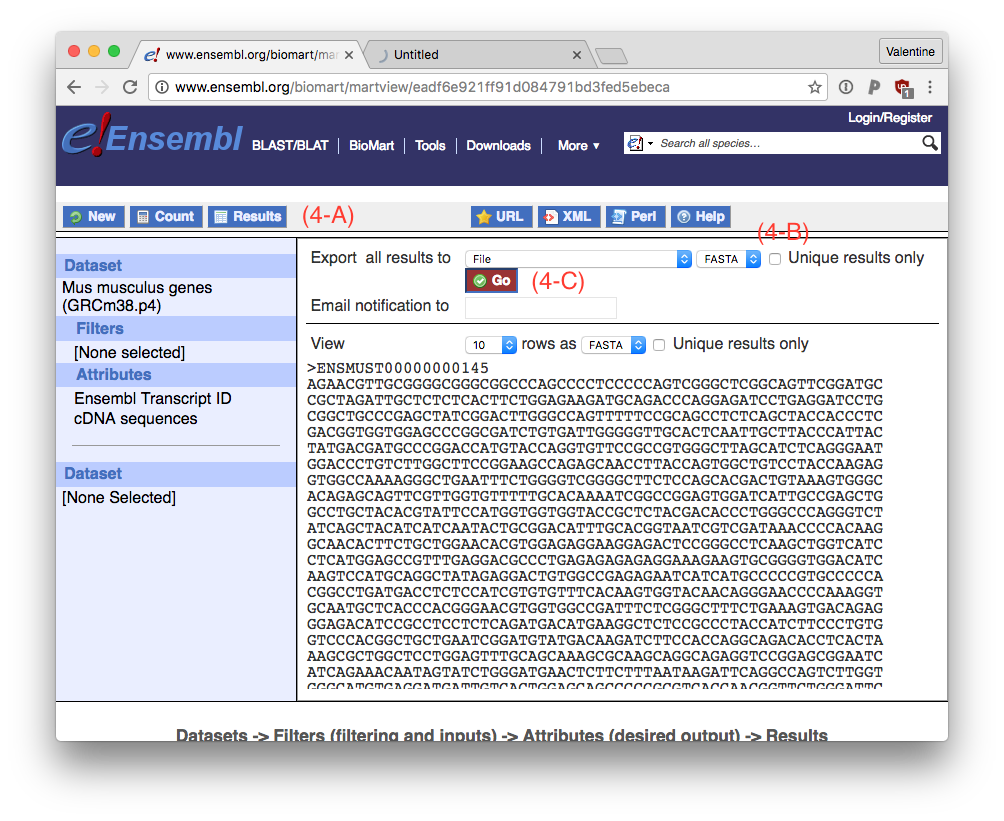
This will download a file called ‘mart_export.txt’, which is about 200 MB large.

We rename this file to something informative so we don’t mix it up with other mart_export.txt files. For me, the informative bits are the genome assembly version and the Ensembl version. As well as an indicator that this is cDNA.

$ cd reference
$ mv mart_export.txt Mus_musculus_GRCm38.p4_E85_cdna.fasta

In many implementation of single cell rna-sequencing spike-ins are added. In this case I am making this example from, we are expecting reads from the ERCC spike ins. These must be added to the reference. Beyond a way to assess success of the experiment, it will also inflate some % reads mapped which is usually used as a quality control metric.

These sequences can be downloaded from https://tools.thermofisher.com/content/sfs/manuals/ERCC92.zip. This is a zip containing ERCC92.fa and ERCC92.gtf, and for this workflow we will only need ERCC92.fa.

The two sequence references files needs to be combined, and this is really simple for FASTA files, you simply catenate them.

$ cat Mus_musculus_GRCm38.p4_E85_cdna.fasta ERCC92.fa > Mus_musculus_GRCm38.p4_E85_cdna_ERCC.fasta

At this point I just want to mention that this might not be enough to cover the cDNA you should expect in a sample. In many cases repeat regions are expressed and gets converted to cDNA. We looked at RNA of repeats in our recent paper in Cell Reports.

There might be other sources of cDNA you might want to add to the reference, like potential contaminants. This can help explain low mapping rates.

In this example I am using Salmon. I would also recommend Kallisto, but at the moment Salmon has the ability to model more biases.

Make sure you have Salmon installed. You can download the binary from github, or install it with Homebrew/Linuxbrew.

To keep track of indices, I like make a directory for the kind of index I am making, then create the index in there.

$ mkdir salmon

Keeping the name the same makes it easier to relate back to what you ran the samples against.

$ salmon index -t Mus_musculus_GRCm38.p4_E85_cdna_ERCC.fasta -i salmon/Mus_musculus_GRCm38.p4_E85_cdna_ERCC.fasta

This takes about 5 minutes.

Salmon can take a ‘genemap’ to summarise expression to the gene level (by summing the expression of transcripts arising from a given gene). The ‘genemap’ is a simple TSV table with gene and transcript name. We get this from biomart as well, to match the cDNA index.

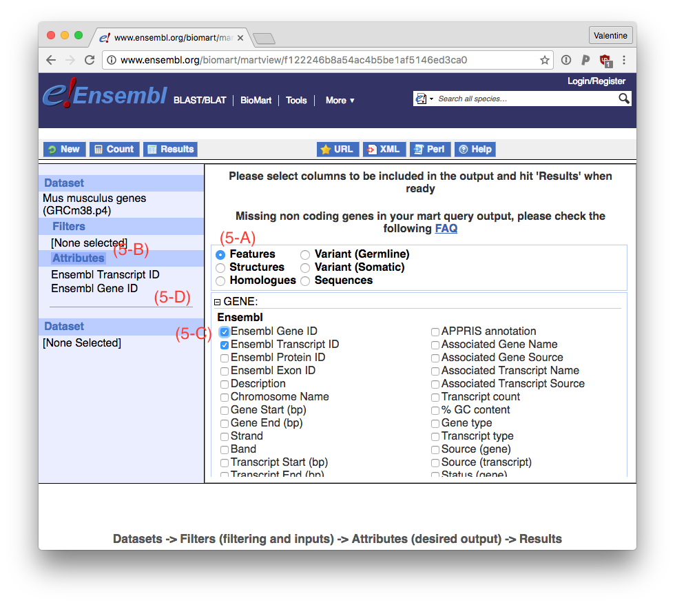
The simplest way to generate this is to go to ‘Features’ (5-A) in the Attributes (5-B) of Biomart. The table need to be ordered (transcript, gene). So unclick ‘Ensembl Gene ID’ (5-C), then click it again, so the order is correct (5-D).

Go to Results (6-A) and download the file as TSV (6-B) by clicking ‘Go’ (6-C).

Rename this text file to something memorable. Again, I like to match the name of this file with the FASTA file to keep track of these belonging together.

$ mv mart_export.txt Mus_musculus_GRCm38.p4_E85_cdna.genemap.tsv

We need to add the ERCC names to this list though. To make a “genemap” from the ERCC FASTA file you can run the following command:

$ grep '>' ERCC92.fa | tr -d '>' | sed 'p' | paste -d '\t' - - > ERCC92_genemap.tsv

Now we can simply merge the mouse cDNA genemap and the ERCC genemap

$ cat Mus_musculus_GRCm38.p4_E85_cdna.genemap.tsv ERCC92_genemap.tsv > Mus_musculus_GRCm38.p4_E85_cdna_ERCC.genemap.tsv

Expression quantification - processing the data

Now let us move to the actual expression quantification. I am going to assume you have a directory with one pair of FASTQ files per sample (one forward and one reverse file per sample). You probably don’t, but the way data is delivered from sequencing facilities is so heterogeneous, you will just have to figure out how to reach this stage. For example, at the Wellcome Trust Sanger Institute, sequencing data is delivered in CRAM files, which need to be converted.

I find it easiest to organise things so that in a data directory of a project, I have one directory with FASTQ files, and make another directory with Salmon outputs, called ‘salmon’. (Or similar for any other program that solves a problem.)

$ cd ..
$ ls fastq/ | head
sc1_cell10_1.merged.fastq
sc1_cell10_2.merged.fastq
sc1_cell11_1.merged.fastq
sc1_cell11_2.merged.fastq
sc1_cell1_1.merged.fastq
sc1_cell12_1.merged.fastq
sc1_cell12_2.merged.fastq
sc1_cell1_2.merged.fastq
sc1_cell13_1.merged.fastq
$ mkdir salmon
$ cd salmon

Now we have everything you need to run Salmon on any given sample. However, this will be tedious, so you should write some script which will do this for you. A very portable way to do this is by using GNU Make. A more intuitive alternative for this sort of processing is to use Snakemake. Below I’m pasting in an example Snakemake file.

$ cat Snakefile
import glob

FASTQS = glob.glob('../fastq/*_1.merged.fastq')

rule all:
   input: [os.path.basename(fq).replace('_1.merged.fastq', '_salmon_out') for fq in FASTQS]

rule salmon:
   input:
       index='../reference/salmon/Mus_musculus_GRCm38.p4_E85_cdna_ERCC.fasta',
       genemap='../reference/salmon/Mus_musculus_GRCm38.p4_E85_cdna_ERCC.genemap.tsv',
       fwd='../fastq/{sample}_1.merged.fastq',
       rev='../fastq/{sample}_2.merged.fastq'
   output:
       '{sample}_salmon_out'
   shell: '''salmon quant -i {input.index} \
                          -l IU \
                          -g {input.genemap} \
                          -1 {input.fwd} \
                          -2 {input.rev} \
                          -o {output} \
                          --posBias \
                          --gcBias
          '''

This Snakefile just runs one command on each sample, which is ‘salmon quant’. Here we provide the reference and the genemape with the -i and -g flags. For Salmon you also need to specify the library type, regarding strand specificity, which is one factor used to judge the mapping locations of read pairs. For ‘normal’ samples this ‘-l’ flag will be IU, but check the documentation to be sure this corresponds to your samples. We also provide some flags to calculate bias parameters. By running ‘snakemake’ in the ‘salmon’ directory you can execute ‘salmon quant’ for all samples. If you have access to a cluster you can run hundreds of these at once by doing e.g. (if you have LSF)

$ snakemake --cluster "bsub -M 10000 -R 'rusage[mem=10000]'" --jobs 200

Once this finishes, you will have expression values for all your samples.

Bringing the data together

What we described above will get you one resulting Salmon directory per sample. To compare these samples, you need to combine the results to a table. As I work mostly in Python, I made a little helper package to combine these to useful tables.

%pylab inline

import readquant

sample_info = readquant.read_qcs('salmon/*_salmon_out', version='0.7.2')

This command parses technical information from the Salmon results which are useful for quality control of the samples. Next read in the expression values per gene in the samples.

tpm = readquant.read_quants('salmon/*_salmon_out')
tpm.iloc[:5, :3]

	salmon/sc1_cell35_salmon_out	salmon/sc1_cell24_salmon_out	salmon/sc2_cell55_salmon_out
Name
ERCC-00158	90.6392	0.00000	0.0
ERCC-00154	35.6046	21.19100	0.0
ERCC-00150	43.4815	0.00000	0.0
ERCC-00143	12.7487	6.95937	0.0
ERCC-00142	0.0000	0.00000	0.0

Now, when we are working on gene level, it is good to generally have an annotation of the genes we are interested in. We have been going back to Biomart a lot but this is the last one! Go Attributes (7-A), then Features (7-B), unclick Ensembl Transcript ID (7-C), then click everything you might be interested in on gene level.

A must is the Associated Gene Name which will allow you to relate the gene id to something recognizable. Chromosome Name is useful for e.g. filtering MT genes. I like the ability to check the rough location of a gene using the Gene Start (bp), for example, if a number of genes are highly correlated, I can quickly check if they are at they share a locus. If there is anything you think you might be interested in relating to the genes you might find, just add it. When you’re done, go to Results (8-A), and download the table as a CSV (8-B) by clicking ‘Go’ (8-C).

Again rename this annotation file so you can relate it to the rest of the files.

$ cd ..
$ mv /Users/vale/Downloads/mart_export\ \(1\).txt reference/Mus_musculus_GRCm38.p4_E85_gene_annotation.csv

Read in this annotation file in the Python you are running

import pandas as pd
gene_annotation = pd.read_csv('reference/mus-musculus/Mus_musculus_GRCm38.p4_E85_gene_annotation.csv', index_col=0)

Beyond the purely technical information, some QC information can be generated based on the abundance estimates. Firstly, the ERCC spike-ins gives some relative information about the mRNA amount captured from a cell. A note is to also remove ERCCs from expression abundances, since this will mask differences in relative mRNA abundance in each cell. Finally, two common metrics for QC are the number of detected genes, as well as the relative abundance of mitochondrially encoded genes.

qc_info = pd.DataFrame(tpm.loc[tpm.index.str.startswith('ERCC-')].sum(), columns=['ERCC_content'])
etpm = tpm.loc[~tpm.index.str.startswith('ERCC-')]
etpm = etpm / etpm.sum(0) * 1e6
qc_info['num_genes'] = (etpm > 1).sum()
qc_info['MT_content'] = etpm.loc[gene_annotation['Chromosome Name'] == 'MT'].sum()
sample_info = sample_info.join(qc_info)
sample_info.head().T

	salmon/sc1_cell35_salmon_out	salmon/sc1_cell24_salmon_out	salmon/sc2_cell55_salmon_out
num_processed	6454761	3848929	2753898
num_mapped	4915485	2605536	1380493
percent_mapped	76.1529	67.6951	50.1287
global_fl_mode	68	57	80
robust_fl_mode	100	100	175
ERCC_content	612303	339921	514.417
num_genes	9575	12073	9005
MT_content	116475	67066.2	3395.65

Now everything is processed, and we can save the files and move on to downstream analysis.

etpm.to_csv('salmon_etpm.csv')
sample_info.to_csv('salmon_sample_info.csv')

From this point, you have expression values and sample information which can be used in the tutorials mentioned above.

As an example, and to end with an actual plot, we could investigate things like mapping rate and number of detected genes:

plt.xscale('log')
plt.scatter(sample_info.num_processed, sample_info.num_genes, c='k');