Swedish School Fires by Gaussian Process Regression — What do you mean "heterogeneity"?

My former colleague Mikael Huss recently published an interesting data set on Kaggle which indicates the school fires reported in Swedish municipalities over last few years. This is coupled with some predictors for the towns over the same years, with aim to see if some predictors associate with an increase in school fires.

The data set is published along with some initial analysis. I was surprised at the poor performance when normalising the fire counts by population, to obtain a frequency.

Partially I got curious about why that was, but also was wondering if I could formulate a nice non-linar model for the data using Gaussian Process Regression.

I registered and downloaded the data from Kaggle. First I read in the fire cases.

%pylab inline
import pandas as pd
import seaborn as sns

Populating the interactive namespace from numpy and matplotlib

fires = pd.read_csv('school_fire_cases_1998_2014.csv')

sns.set_style('ticks')
sns.set_color_codes()
sns.set_context('talk')

Now let's see how these counts relates to population in municipalities

figsize(6, 4)
plt.loglog()
plt.scatter(fires.Population, fires.Cases, c='k', s=30);
sns.despine()
plt.xlabel('Population'), plt.ylabel('Cases');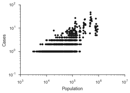

There seem to be a relation, though it looks a bit binary, more clear at the high end where there are around 10 cases. These seem like a bit too few cases per town to beat out stochastic noise. To picture the underlying generative process a bit better, we ignore the time-dimension we have, and just consider the total number of cases in each town in this region.

sum_fires = pd.DataFrame(fires.groupby('Municipality').sum()['Cases']) \
.join(fires.groupby('Municipality').max()['Population'])

plt.loglog()
plt.scatter(sum_fires.Population, sum_fires.Cases, c='k', s=30);
sns.despine()
plt.xlabel('Population'), plt.ylabel('Cases');

Now the relation between the cases of school fires and the population of a town is much clearer!

This indicates that we should be able to normalise the cases succesfully in to a frequency. However, I would prefer putting the population as part of the model, which we will get into later.

First, let us look at our predictors per town. These are referred to as Key Performance Indicators in the data set.

indicators = pd.read_csv('simplified_municipality_indicators.csv')

indicators.columns

Index(['code', 'name', 'medianIncome', 'youthUnemployment2010',
       'youthUnemployment2013', 'unemployment2010', 'unemployment2013',
       'unemploymentChange', 'reportedCrime', 'populationChange',
       'hasEducation', 'asylumCosts', 'urbanDegree', 'satisfactionInfluence',
       'satisfactionGeneral', 'satisfactionElderlyCare', 'foreignBorn',
       'reportedCrimeVandalism', 'youngUnskilled', 'latitude', 'longitude',
       'population', 'populationShare65plus', 'municipalityType',
       'municipalityTypeBroad', 'refugees', 'rentalApartments', 'governing',
       'fokusRanking', 'foretagsklimatRanking', 'cars', 'motorcycles',
       'tractors', 'snowmobiles'],
      dtype='object')

Now, I have been a bit lazy, and I haven't actually read the documentation for these. I don't know the units for these, and which ones are normalised for population. Or which ones it would make sense to do that with.

To quickly get a hang of this, I like to use a trick from computational biology, which is to look at the correlation matrix of these variables, ordered by linkages based on similarity between the correlations.

cmp = sns.clustermap(indicators.corr(method='spearman'), yticklabels=False);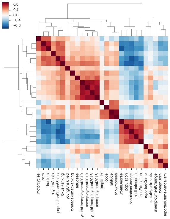

Generally, I don't like putting too much weight in to these linkage clusterings. But we do see two fairly distinct groups. One contains the population variable, so likely the other members of this group are counts rather than frequencies.

(This also shows some entertaining things, like the snowmobiles strongly correlating with latitude.)

Now, we want to use some of these to predict the number of cases of school fire in a given town. Say that $ C $ is the cases of school fire, and that $ P $ is the population. Following this, we let the remaining predictors be $ x_1, x_2, $ etc. The clear relation between $ C $ and $ P $ we noted above, and it would seem we could invsetigate $ \frac{C}{P} $, assuming a linear relation. But we could also behave a bit more agnoistically about this relation.

$$
\log C = f(\log P) + g(\log x_1, \log x_2, \ldots) + \varepsilon
$$

I don't have a particularly good argument for doing all this on a log scale. It is just that I've found it to be generally useful when there are several orders of magnitude of dynamic range.

Ideally here, the effect of population size should be captured by the function $ f $.

An issue though, is the predictors which correlate with population. Since we want all the effects of Population size to be captured in $ f $, we would need to remove this effect from the other predictors. Since we know that Population will predict the Cases quite well, finding one of these to be predictive will most likely just illustrate confounding with the Popultion effect. I can't really think of a clever way of dealing with this (except "normalising" them, but I want to avoid that strategy here, as the point is to try to be non-parametric). For now, we deal with this by not picking predictors from the cluster that correlates with population.

What we actually want to learn is, which of the predictors in $ g $ is more important?

By performing Gaussian Process Regression, we can investigate the functions $ f $ and $ g $. This is a Bayesian technique, where we first provide a prior distribution for each of the functions. If the prior distribution is such that the covariance of function values are parametrised by a covariance function between the predictor values, these distributions will be Gaussian Processes. By selecting your covariance function, you state what kind of functions you would expect if you hadn't observed any data. Once you have observations of data, you can find the posterior distribution of function values for $ f $ and $ g $.

For my research, I use Gaussian Process Regression and other related models to investigate the dynamics of gene expression.

In our case, we will use the Squared Exponential covariance function for $ f $, and an Automatic Relevence Determination version of the SE covariance function for $ g $. The ARD will allow us to find which predictor variables affect predictions from the model, which should relate to their importance.

To model the data as described above, we will use the new Gaussian Process package GPflow. This package implements several Gaussian Process models, and components for these, using the TensorFlow library.

import GPflow

For simplicity, let's combine everything in to one DataFrame.

data = sum_fires.join(indicators.set_index('name'))

data.columns

Index(['Cases', 'Population', 'code', 'medianIncome', 'youthUnemployment2010',
       'youthUnemployment2013', 'unemployment2010', 'unemployment2013',
       'unemploymentChange', 'reportedCrime', 'populationChange',
       'hasEducation', 'asylumCosts', 'urbanDegree', 'satisfactionInfluence',
       'satisfactionGeneral', 'satisfactionElderlyCare', 'foreignBorn',
       'reportedCrimeVandalism', 'youngUnskilled', 'latitude', 'longitude',
       'population', 'populationShare65plus', 'municipalityType',
       'municipalityTypeBroad', 'refugees', 'rentalApartments', 'governing',
       'fokusRanking', 'foretagsklimatRanking', 'cars', 'motorcycles',
       'tractors', 'snowmobiles'],
      dtype='object')

Now we prepare the data for Gaussian Process Regression. We log-scale both the dependent variable, and the predictors (taking care to deal with infinities.)

We also pick some predictors to work with. There are a large number of variables, and with the limited data we have, using all of them will probably just model very small effects which we wouldn't notice very well. Also recall that we don't want to use any of the ones correlating with population!

Y = data[['Cases']] \
        .replace(0, 1) \
        .pipe(np.log10) \
        .as_matrix()

model_kpis = ['Population', 'refugees', 'unemployment2013',
              'longitude', 'asylumCosts', 'satisfactionGeneral',
              'cars', 'fokusRanking', 'youngUnskilled', 'tractors']

X = data[model_kpis] \
        .replace(0, 1) \
        .apply(pd.to_numeric, errors='coerce') \
        .pipe(np.log10) \
        .replace(np.nan, 0) \
        .as_matrix()

A thing which makes these models so flexible, is that the way you express the type of expected functions and the relation between predictors in terms of the covariance function. Here we will formulate the relation by saying that

$$
F(X) = f(\log P) + g(\log x_1, \log x_2, \ldots),
$$
$$
k_F(\cdot, \cdot) = k_f(\cdot, \cdot) + k_g(\cdot, \cdot).
$$

(Here $ k_f(\cdot, \cdot) $ is a covariance function for $ f $ which only acts on the first column of $ X $. And $ k_g(\cdot, \cdot) $ acts on the remaining columns.)

Above, we put the Population in the first column of X, and the remaining columns contain the predicors which we want to use with the ARD SE covariance function.

N_m = len(model_kpis) - 1
kernel = GPflow.kernels.RBF(1, active_dims=[0]) + \
         GPflow.kernels.RBF(N_m , active_dims=list(range(1, N_m + 1)), ARD=True)

Now we are ready to define the model and provide the observed data.

m = GPflow.gpr.GPR(X, Y, kern=kernel)

The way investigate this model, is by selecting hyperparameters for the priors. Hyperparameters are parameters of the covariance functions which dictate features of the functions we are expected to see if we have not observations, which in turn affect the kind of posterior functions we would expect to see.

A nice feature with Gaussian Process models is that in many cases these can be optimized by finding the optimal likelihood of the model. This is also where the power of TensorFlow comes in. Internally in GPflow, you only need to define your objective function, and gradients will be calculated for you.

m.optimize()

compiling tensorflow function...
done
optimization terminated, setting model state





      fun: 47.661120041075691
 hess_inv: <13x13 LbfgsInvHessProduct with dtype=float64>
      jac: array([  2.77119459e-05,   3.10312238e-11,  -5.20177179e-11,
        -1.53390706e-11,  -2.40598480e-10,   7.86837771e-10,
         3.27595726e-04,  -3.28255760e-04,  -3.12000506e-10,
        -1.50492355e-04,   2.20556318e-04,   5.18355739e-05,
        -2.45822687e-03])
  message: b'CONVERGENCE: REL_REDUCTION_OF_F_<=_FACTR*EPSMCH'
     nfev: 154
      nit: 121
   status: 0
  success: True
        x: array([  7.83550523e+00,   4.15028062e+03,   3.49511056e+03,
         8.85917870e+03,   1.25124606e+04,   1.52042456e+03,
         1.27664713e+00,   8.35964994e-02,   5.61225444e+03,
        -1.24241599e+00,   1.31391936e+00,   2.30057289e+00,
        -2.57666517e+00])

After this optimization, we can investigate the model.

Name	values	prior	constraint
model.kern.rbf_2.lengthscales	[ 7.8359016 inf inf inf inf inf 1.52270404 0.73581972 inf]	None	+ve
model.kern.rbf_2.variance	[ 0.25362403]	None	+ve
model.kern.rbf_1.lengthscales	[ 1.55196403]	None	+ve
model.kern.rbf_1.variance	[ 2.39606716]	None	+ve
model.likelihood.variance	[ 0.07327667]	None	+ve

The lengthscale parameters indicate how "dynamic" the function is with respect to the predictor variable. A long lengthscale means that longer distances in the predictor are needed before the function values changes. While a short one means the function values chanes a lot, and thus are sensitive with resposect to the predictor.

The trick of the ARD, is to allow a separate lengthscale for each predictor, but with shares noise. A predictor with a short lengthscale (in the optimal likelihood) will cause many changes as you change the predictor.

This means we can use the inverse of the ARD lengthscales as a measure of variable importance.

pdict = m.kern.get_parameter_dict()
pdict

{'model.kern.rbf_1.lengthscales': array([ 1.55196403]),
 'model.kern.rbf_1.variance': array([ 2.39606716]),
 'model.kern.rbf_2.lengthscales': array([ 7.8359016 ,         inf,         inf,         inf,         inf,
                inf,  1.52270404,  0.73581972,         inf]),
 'model.kern.rbf_2.variance': array([ 0.25362403])}

sensitivity = pdict['model.kern.rbf_2.variance'] / pdict['model.kern.rbf_2.lengthscales'] ** 2

figsize(6, 4)
plt.barh(np.arange(1, N_m + 1) - 0.4, sensitivity, color='k');
plt.yticks(np.arange(1, N_m + 1), model_kpis[1:], rotation=0);
plt.xlabel('Sensitivity');

It is possible illustrate the population effect by itself, by making a Gaussian Process Regression model using only this part of the covariance function, which was optimized for the full model.

i = 8

plt.loglog()

m_pop = GPflow.gpr.GPR(X, Y, kern=m.kern.rbf_1)
XX = np.linspace(3.5, 6.)[:, None]
YY_m, YY_v = m_pop.predict_f(XX)

plt.scatter(10 ** X[:, 0], 10 ** Y, c=10 ** X[:, i], s=40);
sns.despine()
plt.colorbar(label=model_kpis[i])

plt.plot(10 ** XX, 10 ** YY_m, c='r', lw=3, label='Population effect')
plt.plot(10 ** XX, 10 ** (YY_m + 2 * np.sqrt(YY_v)), c='r', linestyle='--', lw=3)
plt.plot(10 ** XX, 10 ** (YY_m - 2 * np.sqrt(YY_v)), c='r', linestyle='--', lw=3);

plt.legend(loc='upper left')

plt.xlabel('Population'); plt.ylabel('Cases');

It is still not perfectly visible how a predictor explains school fire cases when correcting for population. As a visualization, we can remove the mean population effect from the cases, and thus look at how the residuals relate to the predictor of choice.

Y_p_m, Y_p_v = m_pop.predict_f(X)

plt.loglog()
plt.scatter(10 ** X[:, 0], 10 ** (Y - Y_p_m), c=10 ** X[:, i], s=40);
sns.despine()
plt.colorbar(label=model_kpis[i])

plt.plot(10 ** XX, 10 ** (0 * YY_m), c='r', lw=3)
plt.plot(10 ** XX, 10 ** (2 * np.sqrt(YY_v)), c='r', linestyle='--', lw=3)
plt.plot(10 ** XX, 10 ** (- 2 * np.sqrt(YY_v)), c='r', linestyle='--', lw=3);

plt.xlabel('Population'); plt.ylabel('Residual of Cases');

plt.loglog()
plt.scatter(10 ** X[:, i], 10 ** (Y - Y_p_m), c='k', s=40);
sns.despine()

plt.xlabel(model_kpis[i]); plt.ylabel('Residual of Cases');

data.sort_values(model_kpis[i], ascending=False).head()[['Cases', model_kpis[i]]]

  
      Cases
      youngUnskilled
    
      Municipality
      
      Perstorp
      4
      19.1
    
      Haparanda
      2
      17.1
    
      Södertälje
      44
      16.9
    
      Skinnskatteberg
      1
      16.6
    
      Gnesta
      5
      16.0