Some intuition about the GPLVM — What do you mean "heterogeneity"?

Over the last year I’ve been learning about the statistical framework of Gaussian Processes. I’ve been thinking about writing about this for a while, but I feel like I would just decrease the signal-to-noise ratio given the fantastic resources available.

One of my favourite models in the Gaussian Process framework is the Gaussian Process Latent Variable Model (GPLVM). The point of the GPLVM, is that if we have multivariate data, we can simultaneously model every variable with a Gaussian Process. It turns out then that the same way that one can pick hyper parameters for a regression model, we can find optimal, latent, predictor variables for the data.

The leap from regression to the latent variable model is a bit drastic though, so I was trying to think of how we could get some more intuition about this. Let us look at a minimal example. We will use the excellent GPy package for this.

We generate a small number of points (5) on a sine curve, and perform Gaussian Process Regression on this.

import GPy

X = np.linspace(0, np.pi, 5)[:, None]
Y = np.sin(X)

kernel = GPy.kern.RBF(1)
m = GPy.models.GPRegression(X, Y, kernel=kernel)
m.optimize()
m.plot(plot_limits=(-0.1, 3.2));

Now we have a curve which optimally describes the 5 points. Imagine we have a stray 6th point. Say we did 6 measurements, but for one of the points we lost the measurement values. Where could this measurement have happened?

Well, we have the model of the curve describing the data. If we guess the measurement values for the 6th point, we can add that as an observation, and evaluate the likelihood of the regression when including the point.

Let us perform this by guessing some potential points in a 20 by 20 grid around or known observations.

N = 20
xx = np.linspace(0, np.pi, N)
yy = np.linspace(0, 1, N)

ll = []
xxi = []
yyi = []
for i in range(N):
    for j in range(N):
        x = xx[i]
        xxi.append(x)
        Xs = np.vstack((X, np.array([[x]])))
        y = yy[j]
        yyi.append(y)
        Ys = np.vstack((Y, np.array([[y]])))
        ms = GPy.models.GPRegression(Xs, Ys, kernel=kernel,
             noise_var=m.Gaussian_noise.variance)
        ll.append(ms.log_likelihood())

plt.scatter(xxi, yyi, c=ll, s=50, vmin=-1e4,
            edgecolor='none', marker='s',
            cmap=cm.Greys_r);
plt.colorbar(label='log likelihood')
m.plot(ax=plt.gca(), c='r', legend=False,
       plot_limits=(-0.1, 3.2));

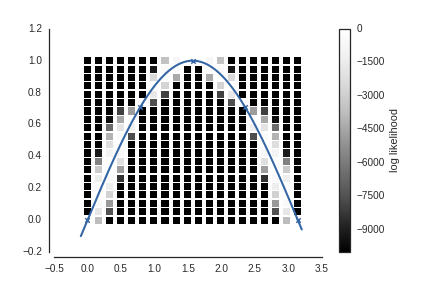
Here every square is a position where we guess the 6th point could have been, colored by the log likelihood of the GP regression. We see that it is much more likely the 6th point came from close to the curve defiend by the 5 known points.

Now, imagine that we know that the y value of the 6th point was 0.4, then we can find an x value such that the likelihood is maximized.

x = 1.2
y = 0.4
Xs = np.vstack((X, np.array([[x]])))
Ys = np.vstack((Y, np.array([[y]])))
gplvm = GPy.models.GPLVM(Ys, 1, X=Xs, kernel=kernel)
gplvm.Gaussian_noise.variance = m.Gaussian_noise.variance
gplvm.fix()
gplvm.X[-1].unfix();

gplvm.optimize()

gplvm.plot(legend=False, plot_limits=(-0.1, 3.2));
plt.scatter([x], [y], c='r', s=40);
ax = plt.gca()
ax.arrow(x, y, gplvm.X[-1, 0] - x + 0.1, gplvm.Y[-1, 0] - y,
        head_width=0.03, head_length=0.1,
        fc='r', ec='r', lw=2, zorder=3);

This is done with gradient descent, and the optimum it finds will in this particular case depend on where we initialize the x value of the 6th point. But if we had more variables than the y value above, and we want to find the x-value which is optimal for all variables at the same time, it will end up being less ambiguous. And we can do this for every point in the model at the same time, not just one.

This is illustrated in this animation.

Here there are two variables and we are looking for x-values which best describes the two variables as independant Gaussian processes.