Unscaling scaled counts in scRNA-seq data

It is always good to compare your measurements with measurements others have done before you. This way you get a feeling for expected outcomes, expected variation in measurement, etc.

In single cell RNA-seq, I tend to apply this principle by looking at a lot of published data, to see how the properties of data in general correspond to data that I’m analyzing for the sake of scientific investigation.

Single cell RNA-seq data consists of observed counts of molecules generated from different genes in different cells. Sometimes however, authors only publish counts that have been scaled. One very popular unit is CPM, counts per million, where the counts in each cell is divided by the sum of counts, then multiplied by a million. Recently I have also noticed data with similar scaling to 10,000 or 100,000, or to a median across the data set.

To compare data from different sources, it is easier to interpret differences if you know the per-cell total counts. It allows you to think of the counts in the data in the context of exposure. I recently wanted to look at some 10X data, but it turned out the expression matrix did not consist of counts.

Looking at the mean-variance relation for all the genes in the data it was clear that they had been log-transformed.

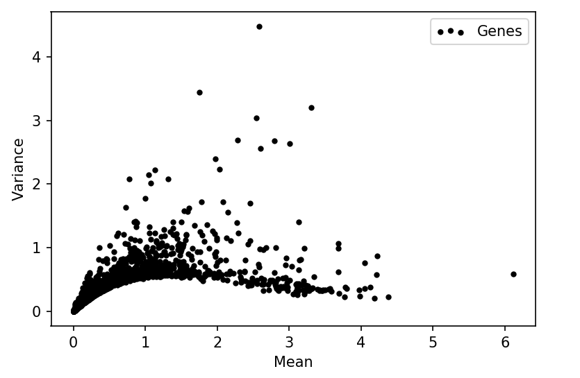
Even after exponentiating the expression levels, they were not integers. However, looking at the sum of expression levels in each cell it could easily be seen that the counts had been scaled to 10,000 counts per cell.

One would think that this is a lossy transformation: we wouldn’t know how large the magnitudes in a cell were before division. However, the very problem with scaling of counts means we can recover the value used to scale the cell.

It’s not clear if this is a biological property or a property of the measurement process, but out of the 20,000 or so genes, in scRNA-seq data of any given cell, the vast majority of genes will have 0 counts. Follows by a substantial number of genes with 1 counts, followed by a slightly smaller number of genes with 2 counts, etc.

Since the scaling by division just changes the magnitude of the counts, but not the discrete nature, the most common value will correspond to 0, the second most common value to 1, etc. This plot of a few random cells make this relation clear.

Just looking at the second most common value in the histogram of a cell will give us the factor used to scale the cell! (For the sake of some robustness, I used several ranks in the histogram and the corresponding scaled counts and fitted the scaling factor with least squares, but the difference from the second most common value was all in all negligible).

By simply multiplying the cells by the identified scaling factors, the true counts are recovered. After un-scaling, the typical relation between total count and detected genes is clear, and the negative binomial mean-variance relation for genes is apparent.

I wanted to write about this, because the fact that it is possible to recover the original counts after scaling indicates that just scaling the counts is not sufficient for normalization. The properties if discrete counts are still present in the data, and will be a factor in every analysis where these scaled counts are used. It will make interpretation hard, since the relation between magnitude and the probability of generating values magnitude will not be tied to each other as clearly as with counts.

Notebook with this analysis is available here.

Resolving immune cell fates in malaria

Malaria is one of the world's deadliest diseases with 200 million cases in a year, leading to half a million deaths. It is caused by mosquito-borne Plasmodium parasites. During parasitic infections our adaptive immune system responds through a complex series of cellular interactions, precipitated by events at the molecular level. The dynamic ability to suppress and activate genes allow immune cells to maintain surprising plasticity. Switching the states of the cells in response to infection require a network of gene regulatory events to occur.

At the heart of the adaptive immune system are T helper cells. Under healthy conditions, naive T helper cells are quiescent and roam through the body awaiting signals. Once T helper cells receive activation signals they differentiate into different roles depending on the type of infection. In malaria, naive cells differentiate into two distinct populations with different roles: Th1 cells, which signal macrophages and killer T cells to attack infected cells. And Tfh cells, which activate survival programs and promote antibody affinity in B cells.

Differentiation into a role is orchestrated by a small number of transcription factors regulating expression of large sets of genes. Identifying transcription factors that direct the differentiation fate is of key importance to understand the immune system, and to what degree in vivo cell-extrinsic factors bias the cell fate has not been studied in detail.

Immunology tightly links cellular biology and molecular genomics. Recently single cell RNA sequencing has gained massive popularity to investigate cells with this joint perspective (1). This technology allows researchers to measure expression of all genes in thousands of single cells. Immune cells however have particularly low amounts of RNA and many important genes, such as transcription factors, are present at low levels. To ensure scRNA-seq would be useful for us we evaluated many different technologies with ground truth molecular input levels (2). To our surprise we found that expression could be quantified even from tens of copies of RNA molecules!

To chart the immune response to malaria we designed a large scRNA-seq time course experiment using a mouse model. We collected T helper cells, monocytes, and dendritic cells from mice infected by the malaria parasite Plasmodium chabaudi at five points over seven days (3).

We used Gaussian process methods to identify and investigate genes with expression dynamics over time. These are nonparametric machine learning models that can represent and identify any smooth dynamic function. (Later we extended this method to identify spatially variable genes in spatial tissue gene expression systems (4).)

Unfortunately five time points are not sufficient to make conclusions about the dynamics of gene expression. However, we could exploit the fact that the immune cells are not synchronized in their response. An extension of the Gaussian process model let us estimate latent per-cell “time points” which could be earlier or later than cell collection times. This Gaussian process latent variable model simultaneously model many genes as different smooth functions, and correct time values so genes are consistent between each other. Now we could investigate the temporally dynamic genes and looked at when they started, peaked, and stopped expression. This way we learn the order transcriptional programs like activation or proliferation.

The most crucial aspect of our experiment was that the T helper cells had two different fates. Meaning any gene’s dynamic expression was the result of either of two functions: a Th1 fate function, or a Tfh fate function. We needed a way to analyse gradual commitment to either fate, without knowing which cells were on which path.

We solved this problem using a mixture of overlapping Gaussian processes. A mixture model is a statistical way to formalize the cell fate assignment problem described above. Machine learning algorithms can be used to infer the most likely groupings of cells into the components of the mixture. In our case cells would be assigned to either a “Tfh component”, or a “Th1 component”, with ambiguous assignments for uncommitted cells.

After fitting the mixture model to assign cells to fates, we could investigate how each individual gene related to the fates. This was the final key to uncovering transcriptional programs for the fate choice. This recapitulated the known Tfh markers Bcl6 and Cxcr5, but in particular let us associate the maintenance of Tcf7 with the Tfh fate. The mixture model identified the Tcf7 antagonist Id2 as the main transcription factor associated with the Th1 fate, along with many known Th1 genes.

The peak times of dynamic genes could be linked to when cells started committing to fates. This identified receptors which were compatible with signaling molecules expressed by the monocytes we had collected in parallel. We confirmed that mice with reduced numbers of monocytes produced smaller fractions of Th1 cells. (Mice with reduced number of B cells on the other hand produce smaller fractions of Tfh cells).

It was possible that T helper cells driven to either fate by the communicating cells had already been primed to respond to only these cells. Using the T cell receptor sequence in the T helper cells as a natural clonal barcode, we found that both Th1 and Tfh cells shared sequences, and must have originated from common naive progenitors.

In summary our data indicate that in malaria activated T helper cells start expressing Tcf7. After proliferation rate acceleration the cells express receptors which receive signals from monocytes or B cells. Cells receiving B cell signals maintain Tcf7 expression and become Tfh cells, while cells receiving monocyte signals replace Tcf7 expression with Id2 expression and become Th1 cells.

Biology is entering a new era with the rich measurements from single cell RNA sequencing. It allows us to use machine learning to ask explicit questions about the data. The power is particularly clear from the joint cellular and molecular perspective. Going forward I hope for more developments that allow us to ask and answer questions from this perspective, and more opportunities for methods like the overlapping mixture of Gaussian processes that can link the two.

References and notes

1. V. Svensson, R. Vento-Tormo, S. A. Teichmann, Exponential scaling of single-cell RNA-seq in the past decade. Nat. Protoc. 13, 599–604 (2018).
2. V. Svensson et al., Power analysis of single-cell RNA-sequencing experiments. Nat. Methods (2017), doi:10.1038/nmeth.4220.
3. T. Lönnberg et al., Single-cell RNA-seq and computational analysis using temporal mixture modeling resolves TH1/TFH fate bifurcation in malaria. Science Immunology. 2, eaal2192 (2017).
4. V. Svensson, S. A. Teichmann, O. Stegle, SpatialDE: identification of spatially variable genes. Nat. Methods. 15, 343–346 (2018).
5. I. C. Macaulay et al., Single-Cell RNA-Sequencing Reveals a Continuous Spectrum of Differentiation in Hematopoietic Cells. Cell Rep. 14, 966–977 (2016).

This post was originally an essay I submitted for a competition on work done in the field of genomics during PhD. Thanks to Sarah Teichmann, Lynn Yi, and Eduardo Beltrame for feedback on the text.

Integrating scRNA-seq and spatial STARmap data from mouse frontal cortex with scVI

In the last few months a number of interesting brain single cell datasets have been published. The new promising STARmap method was pusblished by Wang et al in Science using mouse brain data as example applications. Even more recently, two back to back mouse brain atlases were published in Cell. Zeisel et al characeterized the nervous system of adolescent mice through sequencing over 500,000 cells from 19 different regions using the 10X Genomics Chromium technology. Saunders et al studied adult mouse brain using almost 700,000 cells from 9 regions of the brain using the Drop-seq method.

All three papers contain some data from the frontal cortex region. An interesting exercise is to see how these datasets relate to one another, and if they can be analysed as a single entity.

The Wang et al STARmap data measures a panel of 166 genes in the medial prefrontal cortex (mPFC), across 3,700 cells from three separate biological samples. The STARmap data does not have any clusters annotated, but they do have spatial locations in the tissue preserved! The data from Saunders et al and Zeisel et al are transcriptome wide, so much larger. But it would be interesting to see how well the small panel of STARmap genes would work to integrate and analyse these datasets.

The anterior cortex data from Zeisel et al consists of 14,000 cells with annotations for 53 clusters (though some of these seem to be enteric neurons which is a bit odd?). The frontal cortex dataset from Saunders et al has over 70,000 cells annotated with 62 clusters. For the sake of simplicity, here I randomly sampled 15,000 cells from the Saunders data.

When the datasets are combined we get an expression matrix with 32,000 cells with counts in 158 genes. To analyze the data together I use scVI an autoencoder based method that have been working well in my current research work. Technology specific effects can be accounted for by providing them as batches.

Because we are looking at very few genes here, running inference on the scVI model takes about 10 minutes for 100 epochs. The scVI model then gives you access to a low-dimensional (10 dimensional in this case) latent representation space which can be used to generate counts for all genes consistent with the structure in the original data. The main point with this is that many machine learning and statistical methods that have problems with count data

Once the scVI model is fitted, it is a good idea to create a tSNE of the latent space, and color the cells by various known factors to try to figure out what might contribute to variation in the data.

We see that similar patterns of densities overlap for all the datasets. Of course we need to remind ourselves not to read too much into the tSNE representation; the important part is the 10-dimensional latent representation of the data.

We can note that on the larger annotated scale annotation from the Zeisel and Saunders we can see overlap between related terms in the tSNE! Immune cells close to immune cells, neurons close to neurons, etc.

We can also color the cells by the complete cluster annoation. But with so many clusters it becomes hard to tell the colors apart! (And here I even collapsed some of the Saunders et al cluster names so they would fit in the plot.)

To learn about how the different annotations in the different datasets relate to each other we can use Ward linkage on the cell group centers to create a common dendrogram for all the groups. Because of the design of the latent space, we can simply use Euclidean distances. First we look at the broad cell classes from both the annotated datasets.

From the dendrogram it is clear that the class annotations are consistent between the datasets, as we observed in tSNE above.

We turn then to looking at all 110 annotated clusters in the frontal cortex data from the two publications. This dendrogram is on the larger side, bu the text is stil legible. While it seems pretty consistant within a given dataset, the mixing does not seem completely right. For example neurons in the Saunders et al data are mixed with oligodendrocytes from the Zeisel et l data. This is not necessarily terrible, we are only working with 158 genes from the STARmap panel, the original studies used thousands of genes to define the cell types.

The STARmap cells do not come with cell type annoations. They do however come with spatial locations for every cell! We can try to link the spatial locations in the STARmap data with the cell type annotion in the othe data sets.

scVI has specialized functionality for these tasks, both for semi-supervised learning to annotate cells, and for working with combined spatial and scRNA-seq datasets. Here however we will just do something simple to see how it works out.

Since Euclidean distances are meaningful in the latent 10-d space, we can use a kNN classifier using clusters or classes as targets.

Now we can plot the spatial locations of the STARmap cells, but annotate the cells with predicted clusters from the scRNA-seq datasets. This way we can qualitatively evaluate whether the clusters are consistent with spatial structure in the brain.

In these plots above, each "stripe" consists of different biological samples, and it wouldn't make sense to plot the cells from different biological samples in a single plane. I think they are even from different mice.

From this it seems that prediction to the annotation from Saunders et al seem more spatially organized in the STARmap data.

The cell types in the Zeisel et al data are predicted more spread out in the STARmap data. I suspect there is an issue with the cell type annotation here, since excitatory neurons (TEGLU*) are mapped to the region at the right which is supposed to be non-neuronal. I might have misunderstood how the cell clusters are indexed in the Loom files for cortex. (There is also an odd thing where the website says there are 7,000 anterior cortex cells, but the Loom file contains 15,000).

A notebook with all analysis, including fitting the scVI model, is available here.

Identify tissue structure with Automatic Expression Histology

A while after the invention of the microscope, scientists started applying various chemical dyes when looking at biological samples in the form of tissues from diseased organs. This revealed anatomical structures on the microscopic scale in many plant and animal tissues, birthing the field of histology. Microscopy of stained tissue is still an enormously important field, and histopathologists have devised metrics for diagnosing many types of conditions and diseases based on patterns of cells in stained tissues.

The original classification of the six neuronal layers in the cerebral cortex for example was made on the basis of morphology observed using “Nissl staining” which highlights the endoplasmic reticulum.

Since the original studies of brain microanatomy in the late 19th century we have figured out that the functions and phenotypes of cells (including neurons) are determined by regulation of gene expression programs. Many histological assays are now defined by examining particular gene products examined using immunohistochemical assays.

Researchers are now making extremely rich molecular measurements with preserved spatial coordinates in tissues. At the same time as genome wide measurement are being miniaturized into technologies that preserve spatial location in tissues, technologies for counting individual mRNA molecules in cells using imaging are being increasingly parallelized. We are reaching a point where these two approaches to spatial gene expression analysis are converging to similarly rich assays, with the ability to look at thousands of gene products in thousands of individual cells in tissues.

Similar to how pathologists have defined visual morphological “markers” for cell types in tissues, it is possible to look directly at gene expression or protein abundance throughout the tissue to learn about its structure.

The function of regions of tissues will in many cases be determined by sets of co-expressed genes. This means there is a coupling between spatial locality of function and particular sets of genes.

The automatic expression histology (AEH) model which we published in Nature Methods earlier this year attempts to explicitly model this coupling through a probabilistic model:

$$ \begin{align*} P(Y, \mu, Z, \sigma^2, \Sigma) &= P(Y | \mu, Z, \sigma^2) \cdot P(\mu | \Sigma) \cdot P(Z), \\ P(Y | \mu, Z, \sigma^2) &= \prod_{k=1}^K \prod_{g=1}^G \mathcal{N}(y_g | \mu_k, \sigma^2)^{(z_{g, k})}, \\ P(\mu | \Sigma) &= \prod_{k=1}^K \mathcal{N}(\mu_k | 0, \Sigma), \\ P(Z) &= \prod_{k=1}^K \prod_{g=1}^G \left( \frac{1}{K} \right)^{(z_{g, k})}. \end{align*} $$

Here \( Y \) is a set of vectors of \( G \) genes observed in \( N \) locations in the tissue. The first couple of equations just describe a probabilistic model of clusters: a Gaussian mixture model with \( K \) components. Here the matrix \( Z \) is binary, and only has one non-zero entry per row which assigns an observation to a component. The last two lines though specify that means in the GMM should be generated from smooth spatial functions, thus giving the form of a mixture of Gaussian processes. The covariance matrix \( \Sigma \) encodes spatial locality.

Modeling the spatial functions with Gaussian processes means you do not need to know what they look like, we just assume they are somewhat smooth.

In this model the expression levels of genes are governed by underlying shared spatial functions. The information we know from the experiment is \( Y \) and \( \Sigma \). We don’t know what the functions look like (\( \mu \) and \( \sigma \)) and we don’t know which genes share which function (\( Z \)).

This figure gives a visual representation of the idea of how the binary matrix \( Z \) assigns genes \( g \) to underlying patterns \( k \):

Implemented in the SpatialDE package there is a Bayesian inference algorithm for learning posterior probabilities of the assignments \( z \) between genes and hidden spatial patterns that, together, give rise to spatial co-expression. In our paper we applied it to breast cancer tissue and found a set of immune genes spatially co-expressed in a region of tumor infiltration. We also applied it to mouse olfactory bulb data and got a clear picture of the layer structure of the organ. As well as spatial organization of cell types in a small region of mouse hippocampus.

As a new example here, we can apply the method to an extremely interesting recent dataset that was produced using the novel STARmap technology. This protocol uses in situ DNA sequencing to decode barcodes bound to mRNA molecules within cells of a given tissue, integrating the concepts of CLARITY tissue clearing, in situ FISSEQ, and seqFISH/MERFISH combinatorial gene tagging.

The dataset we use here as an example probed 1,020 genes in in 1,549 single cells over a region of size of about 700 µm by 400 µm in the primary visual cortex of a mouse (corresponding to Figure 4 in the STARmap paper).

First we run the SpatialDE significance test, and find that 101 of the genes significantly depend on spatial locations of the cells in the tissue. To perform AEH, we use these genes and set the characteristic length scale in the tissue. Setting these parameters is not trivial, and here we are a bit helped by domain knowledge. We happen to know that layers are on the order of a couple of 100 µm, and we expect about eight of them. We then set the length scale to be 100 µm and select eight underlying spatial patterns to assign the genes to.

After running AEH we are given assignments of the genes, as well as the underlying spatial function for a pattern, which is evaluated for all the cells in the dataset/tissue.

HPC: hippocampus, cc: corpus callosum, L1-L6: Layers 1 to 6.

Approximately annotating the image by matching it with the figure in the STARmap paper, we see that the patterns learned by AEH match up with the classical layers of the cortex. While we used the number of layers when running AEH, no information about the structure of them were provided to the model. The layer structure that was originally observed by the morphology of stained cells was now automatically identified by the molecular measurements. One way of viewing this is that we now have access to 101 “colors” from the genes, and the “hues” we get by mixing combinations of them in the different layers form patterns that are easy to see computationally.

Compared to other spatial data this dataset is on the larger side, measuring 1500 locations, but even so AEH converges in a reasonable time. Of course the data sets will get larger, but seeing these technologies spread to more research labs is going to be very interesting. The same way many cell types have been discovered by single cell RNA sequencing, many new microanatomical structures will be discovered in many organs using these spatial gene expression methods. I hope tools such as AEH in SpatialDE will be helpful to the fields of tissue and cell biology.

The analysis of the STARmap data can be seen in a Jupyter notebook here.

Thanks to Carlos Talavera-Lópes for feedback on the post.

Count based autoencoders and the future for scRNA-seq analysis

Two recent computational methods, scVI by Lopez et al and DCA by Eraslan & Simon et al, are the most promising methods for large scale scRNA-seq analysis in a while. This post will describe what they do and why it is exciting, and demonstrate the results of running them on three recent datasets.

In almost all cases, to do anything useful in scRNA-seq the tens of thousands of genes measured need to be summarised and simplified. An extremely effective way to summarise many variables through their covariance structure is principal component analysis (PCA). However, scRNA-seq data consists of counts, which have particular behaviours that cause issues with the interpretation and of PCA.

Potential ways of dealing with this is either figuring out how to transform count data to emulate the characteristics of continuous Gaussian data, or to reformulate PCA for the count setting. While data transformations have historically had some success, they don’t perform so well for low count numbers, which is the case when massive scRNA-seq experiments are economically feasible.

A couple of years ago Risso et al successfully created a generalized linear factor analysis model for scRNA-seq counts called ZINB-WaVE, based on a zero-inflated negative binomial (ZINB) count distribution. Omitting some further features, in this model underlying rates of observations of mRNA molecules from specific genes are modelled by a low-dimensional collection of continuous factors. Every cell has a particular hidden value for these factors, and to fit the model all cells are investigated and assigned the most likely factor values. (In these equations, red color indicates parameters that need to be inferred.)

$$ \begin{align*} Y &\sim \text{ZINB}(\mu, \phi, \pi) \\ \log \mu &= {\color{red}{W}}^{T} {\color{red}{X}} \\ \cdots \end{align*} $$

With these ZINB based methods, the data does not need to be scaled, nor normalised, and in principle the common step of selecting highly variable genes is not necessary. The data just plugs in.

Inherently, learning the \( X \) means that each cell is compared to all other cells. The factors (\( W \)) can be investigated in attempts to deduce meaning, and in that way we gain knowledge. But if you show the model a new cell \( y \), it doesn’t know what to do with it. The inference will need to be rerun with the entire dataset including this new cell.

Two new methods, called scVI (single cell variational inference) and DCA (deep count autoencoder) rethinks this model, by moving from factor analysis to an autoencoder framework using the same ZINB count distribution. (Their titles and abstracts phrase them as imputation methods, which is a bit odd and substantially undersell them!) The two methods have slightly different parameterizations, but conceptually (abusing notation a bit), this represents with they both do:

$$ \begin{align*} Y &\sim \text{ZINB}(\mu, \phi, \pi) \\ \log \mu &= f_{\mu}(X; {\color{red}{\theta_f}}) \\ \cdots \\ \hat{X} &= g(Y; {\color{red}{\theta_g}}) \end{align*} $$

A parametric function from the observed space (gene counts) to a low-dimensional space is fitted (\( g \)), at the same time as a function that maps the low dimensional space to ZINB parameters (\( f \)). For any given cell, you can apply \( g \) to get its \( X \)-representation, then apply \( f \) on that to get parameters, and evaluate the likelihood of the cell. The functions \( g \) and \( f \) are parameterised as neural networks because these are flexible and efficient.

This unlocks a lot of benefits. For inference, this setup makes it easier to use stochastic optimization, and is directly compatible with inference on mini-batches: you only need to look at a few cells at a time, so no matter how many cells you have, you will not run out of memory. Scientifically, this allows you to generalize. You can apply \( g \) to any new cell and see where it ends up in the \( X \)-space.

By analysing how different regions of the \( X \)-space map to gene expression, markers and differential expression can be investigated. And on the converse, if you perform clustering in the \( X \)-space, you can take new cells and evaluate which clusters the \( g \) function maps them to.

To illustrate what the methods do, we will apply them to three recent datasets. I picked smaller datasets on the order of ~2,500 cells because I wanted to quickly run them on desktop just for testing. One from Rosenberg et al 2018, where I randomly sampled 3,000 out of 150,000 developing mouse brain cells. The second one is a taxon of Peripheral sensory neurons from mousebrain.org, which is part of Zeisel et al 2018. And finally a dataset of male mouse germ cells that I found on GEO, but I couldn’t find an associated paper for (Lukassen 2018). I ran both DCA and scVI with default parameters: DCA produces a 32-dimensional representation, and scVI a 10-dimensional. To qualitatively inspect the results I ran tSNE on the representations, and colored the cells based on labels provided from the data sources.

The DCA method is implemented around the anndata Python package, and is very easy to run on any data you have. The scVI implementation requires you to manually wrangle your data into TensorFlow tensors with correct data types, which can be frustrating if you are not used to it. This does however imply that if you want to scale the inference using out-of-core strategies, scVI directly supports that.

In terms of run time, DCA was much faster than scVI, finishing in a few minutes. scVI took about an hour for each dataset. A large component is probably that DCA implements automatic early stopping, while scVI will run for as many epochs as you tell it, even if the fit doesn’t improve.

The scVI method has the option to account for discrete nuisance variables (batch effects), but I did not try this. And even without it, it seems to align the two mice quite well in the Lukassen 2018 data!

I am curious if there is a way to also account for continuous nuisance parameters (e.g. amplification cycles). In ZINB-WaVE this is straightforward, because it is a GLM, but it is not so clear here. I mentioned clustering in the X-space, it might be possible to formulate these models as structured autoencoders (SVAE), and encourage the \( g \) function to learn a representation that favours cell type segmentation. Notebooks where I ran the methods on the different datasets are available here.

Illustrating spatially variable genes with a 1-dimensional zebrafish

The other day SpatialDE, our statistical test for spatially variable genes in spatial transcriptomics data was published in Nature Methods. The goal of the method is to find genes which in some way depend on the spatial organization of tissues, and for our paper we analysed generated with Spatial Transcriptomics, SeqFISH, and MERFISH. As a demonstration of how to use SpatialDE I also analysed some recent heart tissue. The underlying principle in SpatialDE can be hard to get to grips with, and the aim of this post is to provide an example that hopefully explains it.

One very practical reason it can be hard to see what is going on is that it is generally difficult to make plots to visualize data in more than 2 dimensions so that noise is easily interpreted. In terms of spatial gene expression, it is then easiest to make an example with a 1-dimensional tissue, and illustrate things that way.

There is actually a spatial transcriptomics dataset which is in fact 1-dimensional! In a study by Junker et al, the authors studied zebrafish embryos at the 15 somites stage by straightening them, then segmenting them into about 100 slices, each roughly 18 µm thick. For each slice digital RNA sequencing was performed providing expression levels for the entire transcriptome, annotated with the head-to-tail coordinates of the slice: a protocol they call “tomo-seq”. This provides an excellent example to illustrate what SpatialDE mean by “spatially variable genes”.

Defining spatial gene expression

Without pre-specifying the shapes of gene expression we need a way to express properties of how genes could behave across the coordinates. An effective way to look at this is to consider spatial coordinates as locally informative. If you know expression in a coordinate, then nearby coordinates should be pretty similar, while coordinates further away are still somewhat similar. In statistical terms, we say that coordinates \( x_i \) and \( x_j \) covary in a way that decreases with distance between \( x_i \) and \( x_j \). A common way to express this is through the Gaussian covariance function: \[ cov(x_i, x_j) = \exp \left(-\frac{|x_i − x_j|^2}{2 \cdot l^2}\right) \]

The parameter \( l \) describes the scale at which expression levels are locally similar. We illustrate the meaning of this by considering a length scale of 126 µm in the zebrafish embryo.

In this example, we don’t know what the expression values are in any coordinate, but we expect that expression levels 5 slices apart from each other will have a correlation of about 0.8, while expression levels 10 slices apart will have a correlation of about 0.4. In other words, genes may be expressed in or close to the head while not expressed at all in the tail, or vice versa. The right side of the plot shows a couple of expression curves drawn from a multivariate normal distribution with this covariance matrix.

\[ \begin{align*} y_g &\sim \mathcal{N}(0, \Sigma), \\ \Sigma_{i, j} &= cov(x_i, x_j) \end{align*} \]

Models like this where the covariance between points are parameterized are known as Gaussian processes.

Spatial and non-spatial variance

The curves above are random draws, but have you ever seen data that looks so clean? More likely there is additional noise which we cannot explain by only considering the spatial covariance between zebrafish slices. This can be expressed as \[ y_g \sim \mathcal{N}(0, \sigma^2 \cdot (\Sigma + \delta \cdot I)) \]

The \( \sigma^2 \) parameter is the overall magnitude of the variance of \( y_g \), while the \( \delta \) parameter scales how much of the variance not determined by spatial covariance. With these quantities (together with a correction for the structure of \( \Sigma \) called the Gower factor \( G(\Sigma) \)) we can move to a measure we refer to as “fraction spatial variance” (FSV), FSV \( = G(\Sigma) / (G(\Sigma) + \delta) \). This is a number between 0 and 1 which indicate how much of the variance in data is due to spatial covariance. To illustrate, we can randomly simulate data with different levels of FSV.

The simulated data in the panels have the same variance. But we can see that the spatial contribution to the variance decreases as the FSV decreases.

The SpatialDE test fits the \( \sigma^2 \) and \( \delta \) parameters to each genes observed expression levels, and also compares the likelihood with a model that has no spatial variance (FSV = 0) to obtain a significance level (p-value). This way it is possible to distinguish between genes with high variance and genes with high spatial variance. The \( l \) hyper-parameter for the \( \Sigma \) matrix is also fitted through grid search, so for each gene we also get the optimal length scale. (This dataset had 95 samples of 20,317 genes, and the SpatialDE test took about 5 minutes to run).

As an illustration, let us look at the expression patterns of a number of genes identified with different FSVs in the zebrafish embryo.

For the higher FSVs it is clear the expression depends on spatial location, while this is less clear for small FSVs. We can look at the relation between total variance and spatial variance, and how the FSVs are distributed compared to these.

On the right side the standard plot from SpatialDE illustrates the relation between the FSV and the statistical significance for all genes. I put in references to the genes I used as examples, as well as some genes that were highlighted by Junker et al in the original paper. In total SpatialDE identifies 1,010 genes as significantly spatially variable, with most of those genes having length scales between 65 µm and 244 µm.

Hopefully this one-dimensional example helps clear up what we mean by “spatially variable genes”, and also illustrate that there are many forms of data that can use spatial analysis. If you have spatial gene expression data, I recommend trying SpatialDE to identify genes of interest. The analysis associated with this post is available in a notebook here. If you want to use SpatialDE for your spatial data, you can install it by pip install spatialde. Thanks to Lynn Yi for editorial feedback on this post.

Actionable scRNA-seq clusters

Recently Jean Fan published a blog post about "real" scRNA-seq clusters. The general idea is that if there is not differential expression between clusters, they should be merged. This is a good idea, and putting criteria like this highlights expectations of what we mean by clusters, and may in the future direct explicit clustering models that incorporate these.

The workflow Jean presents is similar to how I have been looking at these things recently, and the post inspired me to 1) write down my typical workflow for cell types or clusters, and 2) put my code in Python modules rather than copy-pasting it between Notebooks whenever there's new data to look at. Of course in this post I'll be making commands and images much more stylized than they would typically be, but the concept is representative.

Simulated data

To assess whether an approach is reasonable, it is good to make some simulations of the ideal case. To simulate cells from different cell types, I make use of 1) a theory that cell types are defined by "pathways" of genes, and 2) observations from interpreting principal component analysis from many datasets. These indicate that to produce a transcriptional cell type, a small number of genes are upregulated and covary among each other.

With this in mind, simulation is done by, for each cell type, creating a multivarate normal distribution for each cell type, which have increased mean and covariance for a defining "module" of genes. From this distribution a number of cells are sampled, and expression values are pushed through a softplus function to immitate the nonnegative scale and properties of log(counts + 1). The process is repeated for each cell type, leaving a number of genes as inactive background.

In this particular case I simulate 10 cluster spread over 1,000 cells, with 20 active marker gene per cluster, and finally add 300 "unused" genes.

from NaiveDE import simulate data = simulate.simulate_cell_types(num_clusters=10, num_cells=1000, num_markers_per_cluster=20, num_bg_genes=300, marker_expr=1.8, marker_covar=0.6)

Here a tSNE plot is used as a handy way to look at all the cells at once. The most unrealistic part of this simulation is probably the uniform distribution of cell numbers per cell type. In real data this is very uncommon.

To cluster cells it is pretty effective to work in the space of a number or principal components. I like to use Bayesian Gaussian mixture models to group cells into clusters in this space. First I will cluster with an overly large number of clusters.

from sklearn.decomposition import PCA pca = PCA(15) Y = pca.fit_transform(data) from sklearn.mixture import BayesianGaussianMixture def get_clusters(K): gmm = BayesianGaussianMixture(K, max_iter=1000) gmm.fit(Y) c = gmm.predict(Y) return c c = get_clusters(25)

In this tSNE plot each color correspond to a cluster. As Jean points out, for a cluster to be useful in followup experiments we must be able to define it with a small number of genes. That is, there should be some genes which will allow us to predict whether a particular cell belongs to the cell type or not. For many this is a bit reductionist, and t is not impossible functional cell types are defined by hugely complex nonlinear interactions of hundreds of genes. But in practice, we wouldn't know what to do with such cell types.

The definition of an actionable cell type being one we can predict leads to predictive models. In particular regularised logistic regression is good for this. By controlling the regularisation) so that each cluster has a "marker budget" of only a handful genes, we can ensure that a few markers can predict the types. It is very rare to look at more than ~5 top genes when assessing clusters in practice.

ROC curves from the predicted assignment probabilites in logistic regression is a practical way to assess whether we are able to predict the cell types correctly. Here I split the data into 50% training and testing, train logistic regression, then create the ROC curve for the test data, for each cell type.

The printed numbers in the training command are the number of positive markers for each cell type. I interactively change the sparsity parameter to keep these numbers generally low. In this regard this is all quite supervised and subjective, and far from automated.

from NaiveDE import cell_types test_prob, test_truth, lr_res, lr = cell_types.logistic_model(data, c, sparsity=0.5) [26 24 34 31 8 31 10 10 42 24 17 8 10 39 17 39 5 7 12 7 21 19 10 9 14] cell_types.plot_roc(test_prob, test_truth, lr)

The colors of the curves here correspond to clusters. A number of the clusters are relatively close to the unit line, indicating that we have a hard time predicting these, and they will not end up being actionable. So we decrease the K and try again. We iterate this procedure until we are happy with the predictability of the clusters.

Here I have also plotted cases of "under clustering" the data. The larger clusters are still pretty predictice, but we would want to maximize the number of clusters which would be experimentally actionable.

In the case of K=10 (which is what we simulated), we can also look at which genes the predictive model is using for each cell type. We can use the get_top_markers command to extract the N largest weights for each class in a handy table.

top_markers = cell_types.get_top_markers(lr_res, 5)

To visualise how these weight relate the expression of cells with different cluster annotations, we can plot a "marker map", which sorts cells by cluster, and plots the top marker genes in corresponding order on the Y axis. This is a very common plot in scRNA-seq cluster studies.

cell_types.plot_marker_map(data, c, top_markers)

We see that structure we simulated is largely recovered! The diagonal blocks indicate genes which predict the cell types.

Application to bone marrow data

Now we try this strategy on real data. In particular, we are using one of the batches of bone marrow data from the recently published Mouse Cell Atlas. This batch has 5,189 cells and expression values for 16,827 genes. For the sake of speeding up the analysis a little I randomly sample 3,000 of the cells.

Now we perform the same procedure of training GMM's and attempting to predict held out data with logistic regression.

At 7 clusters I stop, here the clusters are very easy predict. Again we can create the marker map.

Obviosuly this is a lot noisier than the simulated data. Another thing we notice is that the number of cells per cluster is much less even than for the simulated data. This will cause some issues with interpreting the ROC curves, but in practice we want to try to have some minimal size for clusters in order to keep them reliable.

In order to quickly interpret the clusters, and read out what the predictive genes are, the plot_marker_table command will lay out predictive weights and names of top marker genes for each cluster, the colors relate to the colors in the plots.

cell_types.plot_marker_table(top_markers, lr)

I find this workflow fairly straightforward and quick to work around. There are some clear drawbacks of course: tt is quite manual, and we are not quantifying the uncertainty of these predictive weights, so we can't do proper statistics.

Notebooks for this post are available here.

The effect of Poisson zeros on OLS regression results

In a previous post I wrote about the Poisson distribution seeming like a good error model for scRNA-seq counts. This suggests using GLM with Poisson likelihood to analyse your data, as long as the offset due to count depth variation is taken into consideration.

An alternative strategy could be to transform the counts to roughly normal, and perform analysis in that setting. This is effectively what the vast majority of studies do for unsupervised analysis: counts are transformed, then PCA is used to find a low-dimensional representation for further analysis such as clustering.

What if we try to adjust for the count depth variation in a supervised setting assuming Gaussian noise?

A huge benefit of assuming Gaussian noise is that linear regression has an extremely efficient solution, usually referred to as OLS regression. A couple of years ago I made a simple Python package NaiveDE to perform OLS regression on gene expression matrices. I don't recommend anyone use it for final analysis, indeed I called it "Naive DE" because it is a baseline. Literally every other DE test will be better than it by design, in particular with regards to false positive P-values. (Well maybe not according to a recent study, the test in NaiveDE should be equivalent to the t-test.) It is nevertheless convenient during exploratory analysis to iterate through models

Alternative and null models are specified by Patsy formulas, and significance is calculated with a likelihood ratio test. A Bonferroni corrected version of the P-value is also reported.

For every gene \( g \) where we have a design matrix \( X \) and observed counts \( y_g \) we look at

$$ y_g = \mathcal{N}\left( \alpha^T_g X, \sigma^2_g \right). $$

The weights \( \alpha \) are calculated by OLS, and \( \sigma^2 \) is reflected in the residual errors. For flexibility, intercept is optionally part of the design matrix.

Negative control data

In the negative control 10X dataset from Svensson et al 2017, the only variation in observed expression should (in theory) be due technical effects, in particular the count depth variation. Here we are using 2,000 cells with 24,000 genes. The most common variance stabilizing transformation of scRNA-seq data is \( \log(Y + 1) \), so we will investigate how this affects regression.

If the gene counts are scaled per cells, we would want

$$ \log\left( \frac{y_g}{\text{counts}} \right) = \log(y_g) - 1.0 \cdot \log(\text{counts}) = \mathcal{N}(0, \sigma^2) $$

We set up a model where the design matrix \( X \) have the log total counts, and an intercept. Ideally the weights for the log counts should be found to be 1, and the intercept 0. Note that in practice we are always using \( \log(y_g + 1) \).

%%time lr_results = NaiveDE.lr_tests(sample_info, np.log1p(counts.T), alt_model='~ np.log(total_count) + 1', null_model='~ 1')

CPU times: user 2.98 s, sys: 702 ms, total: 3.68 s
Wall time: 3.35 s

The test produces a table with weights from the alternative model, hypothesis test restults.

print(lr_results.sort_values('np.log(total_count)', ascending=False).head(25))

                Intercept  np.log(total_count)           pval           qval
gene                                                                         
ENSG00000198938  -5.501025             1.080920  3.073563e-294  6.147125e-291
ENSG00000198727  -5.600405             1.041435  3.073563e-294  6.147125e-291
ERCC-00002       -2.999032             1.034389  3.073563e-294  6.147125e-291
ERCC-00136       -4.155633             1.017020  3.073563e-294  6.147125e-291
ERCC-00113       -4.297474             1.010625  3.073563e-294  6.147125e-291
ENSG00000198886  -5.615521             1.010178  2.134557e-266  4.269114e-263
ENSG00000198712  -5.144020             1.005586  3.341643e-168  6.683285e-165
ERCC-00096       -2.740023             0.989442  3.073563e-294  6.147125e-291
ENSG00000210082  -4.357098             0.988333  3.073563e-294  6.147125e-291
ERCC-00046       -3.727992             0.979269  3.073563e-294  6.147125e-291

In this plot np.log(total_count) does not refer to the value, but weight for this variable. Each dot is a gene rather than droplet. The P-value comes from comparing the model with one that does not consider the depth.

The marjority of genes are found to have gene count weights much smaller than 1. It turns out that lowly abundant genes will have delfated total count slopes.

We can look at a few examples of genes with different count depth weights.

From this, it is clear that increased observations on the low count values, in particular 0, are responsible for decrease in the total count weight.

Differential expression

Now let us investigate how this count depth effect plays in to a differential expression analysis. With all published large scale experiments cataloging cell types, it is getting increasingly easy to simply fetch some data and do quick comparisons. We will use data from the recent single cell Mouse Cell Atlas30116-8). To get something easy to compare, we use the samples called "Brain" and focus on the cells annotated as "Microglia" and "Astrocyte". Out of the ~400,000 cells in the study, these two cell types have 338 and 199 representative cells. On average they have about 700 total UMI counts each, so while the entire study is a pretty large scale, the individual cell types and cells are on a relatively small scale. The final table has 537 cells and 21,979 genes.

print(sub_samples.head())

                            ClusterID Tissue    Batch        Cell Barcode  \
Cell name                                                                  
Brain_1.AAAACGCGAGTAGAATTA   Brain_3  Brain  Brain_1  AAAACGCGAGTAGAATTA   
Brain_1.AAAACGGAGGAGATTTGC   Brain_3  Brain  Brain_1  AAAACGGAGGAGATTTGC   
Brain_1.AAAACGGGCTGCGACACT   Brain_2  Brain  Brain_1  AAAACGGGCTGCGACACT   
Brain_1.AAAACGGTGGTAGCTCAA   Brain_3  Brain  Brain_1  AAAACGGTGGTAGCTCAA   
Brain_1.AAAACGGTTGCCATACAG   Brain_3  Brain  Brain_1  AAAACGGTTGCCATACAG   

                                    cell_type super_cell_type  is_astrocyte  \
Cell name                                                                       
Brain_1.AAAACGCGAGTAGAATTA  Astrocyte_Mfe8 high       Astrocyte          True   
Brain_1.AAAACGGAGGAGATTTGC  Astrocyte_Mfe8 high       Astrocyte          True   
Brain_1.AAAACGGGCTGCGACACT            Microglia       Microglia         False   
Brain_1.AAAACGGTGGTAGCTCAA  Astrocyte_Mfe8 high       Astrocyte          True   
Brain_1.AAAACGGTTGCCATACAG  Astrocyte_Mfe8 high       Astrocyte          True   

                            total_count  gene  
Cell name                                      
Brain_1.AAAACGCGAGTAGAATTA       1088.0     0  
Brain_1.AAAACGGAGGAGATTTGC        967.0     0  
Brain_1.AAAACGGGCTGCGACACT        543.0     0  
Brain_1.AAAACGGTGGTAGCTCAA        679.0     0  
Brain_1.AAAACGGTTGCCATACAG        957.0     0

In a differential expression test you simply include a covariate in the design matrix that informs the linear model about the different conditions you want to compare. Here we are comparing microglia and astrocytes.

%%time lr_results = NaiveDE.lr_tests(sub_samples, np.log1p(sub_counts.T), alt_model='C(is_astrocyte) + np.log(total_count) + 1', null_model='np.log(total_count) + 1')

CPU times: user 705 ms, sys: 136 ms, total: 841 ms
Wall time: 707 ms

print(lr_results.sort_values('pval').head())

         Intercept  C(is_astrocyte)[T.True]  np.log(total_count)  \
Atp1a2   -1.925596                 1.840452             0.318532   
Sparcl1  -1.008002                 1.742278             0.179123   
Tmsb4x   -3.680027                -2.044908             0.948016   
Hexb     -2.165802                -2.032087             0.646263   
Ctss     -1.665139                -1.937761             0.553429   

                pval           qval  
Atp1a2   3.058918e-162  1.642639e-159  
Sparcl1  3.548817e-158  1.905715e-155  
Tmsb4x   2.742131e-153  1.472524e-150  
Hexb     3.671724e-145  1.971716e-142  
Ctss     8.167943e-144  4.386185e-141 

Also in this case we can see that the count depth weights are deflated for lowly abundant genes.

Similar to above, we can look at the relation between count depth and observed counts for a few genes, but we can also make sure to plot the stratifiction into the two cell types and how the regression models are predicting the counts.

Again we can see the overall abundance is related to the slope of the lines. Another thing which seem to pop out in these plots is an interaction between cell type and slope. For example looking at C1qa the slope for the microglia seem underestimated. This makes sense, if this is an effect of count noise at low abundances.

My takeaway from this is that OLS regression might be OK if counts are large, but at lower levels model parameters are not estimated correctly due to the count nature of the data.

Notebooks of the analysis in this post are available here.

Count depth variation makes Poisson scRNA-seq data Negative Binomial

In the scRNA-seq community the observation of more zero values than expected (called the "dropout problem") is still a concern. The source seems to be an intuition that at such small scales of biological material as RNA from individual cells, molecular reactions lose efficiency due to conceptual stochastic events. The trendiest computational research directions in the field at the moment are probably tied between "how do we do this for a million cells?" and "how do we deal with the dropouts?". In particular droplet based scRNA-seq methods are considered to have more dropouts, often leading investigators that opt for more expensive plate based methods even for exploratory pilot experiments.

In negative control data there is no evidence for zero inflation on top of negative binomial noise, counter to what is commonly suggested (in particular for droplet based methods). A notion that has inspired significant research efforts. A recent interesting report by Wagner, Yan, & Yanai goes even further and illustrates that the Poisson distribution is sufficient to represent technical noise in scRNA-seq data. The authors write that additional variation in gene counts is due to efficiency noise (an observatin from Grün, Kester, & van Oudenaarden that different tubes of reagents appear to have different success rates), and can be accounted for by an averaging approach.

This can be explored by simulating data! Say droplets contain transcripts from 300 genes, whose relative abundance levels are fixed because they come from the same RNA solution. Then a droplet with \( d \) transcripts can be seen as a draw from a multinomial distribution,

\[ c_i \sim \text{Multinom} (d, (p_1, \ldots, p_{300})). \]

Now each gene will independently conform to a Poisson distribution.

The constant mean-variance relation for Poisson holds (as expected) for this simulation. In actual data, genes with higher abundance are over dispersed, which can be modeled using a negative binomial distribution.

The negative binomial distribution is constructed as a mixture of Poisson distributions, where the rate parameter follows a Gamma distribution. Other Poisson mixtures have also been suggested for scRNA-seq data.

An aspect of real data which our mutlinomial simulation does not account for is that the total counts observed in each droplet is variable. Indeed, usually a cutoff at some low number of total counts per droplet is used to decide which droplets captured cells and which only contain background material that is not of interest.

Thinking about the abundance levels of the different genes as rates in Poisson distributions require each observation to come from a constant count depth. If the count depth varies in each observation but the model is not informed of this, it will appear as if the rate for each gene is variable, and this will be more consistent with a negative binomial distribution.

As an illustration, in the simulation, variation in count depths can be included. For simplicity, a uniform distribution is used,

\begin{align} d_i & \sim \text{Uniform}(5.000, 100.000), \\ c_i & \sim \text{Multinom} (d_i, (p_1, \ldots, p_{300})). \end{align}

These new values clearly have the quadratic polynomial mean-variance relation that is typical for scRNA-seq counts.

This indicates we need to handle the differences in count depth. The easiest solution is to simply divide the expression counts in each cell with the total depth, turning each expression value into a fraction.

In the RNA-seq field it is also common to also multiply these fractions by 1 million to form the "CPM" unit.

It is clear that after creating either fractions or CPM will follow a linear relation between mean and variance. However, in both cases there is an offset from the unit relation, and in particular for the CPM unit the variance gets inflated compared to the mean.

The thrid panel shows the result after manually scaling the fractions (through multiplication by 3.5e4) to achieve the Poisson mean = variance relation. (There is probably a closed form expression for the scaling factor that achieves this, and the 1e6 is above this, explaining the variance inflation.)

It is entirely possible that the this type of scaling to create CPM from fractions is one reason people have noticed higher than expected numbers of zeros. For Poisson data, the expected number of zeros at a given mean expression level is given by the function \( e^{-\mu} \).

The counts themselves follow the theoretical curve quite close, but with an increase of zeros at high expression levels, consistent with negative binomial zeros. 'Fractions' see a large offset of much fewer zeros than is expected given the mean, while CPM see an offset for more zeros than expected. The manually scaled values follow the theoretical curve decently, though far from exactly.

For interpretable analysis, counts should be scaled for total count depth, but this also need to be taken under consideration when looking at the results (e.g. dropout rate). The best solution might be to take inspiration from the field of generalised linear models. In that field offsets are included in models when there is a clear explanation for variation in counts, to convert counts to rates. Clustering or pseudotime methods could be reformulated to the Poisson setting with offsets.

There are some additional aspects to keep in mind. For negative control data where each droplet contains RNA from the same solution, the count depth variability must be technical, but in real samples this could also be due to cells having variable amounts of RNA. For droplet based data one simple reason for the heterogeneity could be due to variation in coverage for DNA oligos on barcoded beads. It is not clear what an explanation for plate based methods would be, and no proper negative control data exist for plate based methods to investigate these properties. On a similar note, the latest single cell sequencing methods based on stochastic schemes for in situ barcoding of cells are impossible to assess with negative control samples.

An R notebook for this analysis is available here. Thanks to Lior Pachter for editorial feedback on this post.